Exercise 3: Permeability and Tvent

We now understand a bit better why the approx. 400°C fluids are rising towards the surface and the hotter fluids are remaining stagnant within the reaction zone. Let’s do the next step and understand what is happening at the interface between lower and higher permeabilities.

Go back to our two-layered case and post-process the solution in paraview a bit more.

Load the layered case with constant

Use the paraview calculator to create a two new variables T_Celsius (by doing T_Celsius = T - 273.15) and mass flux (U*rho)

Make a z-normal slice

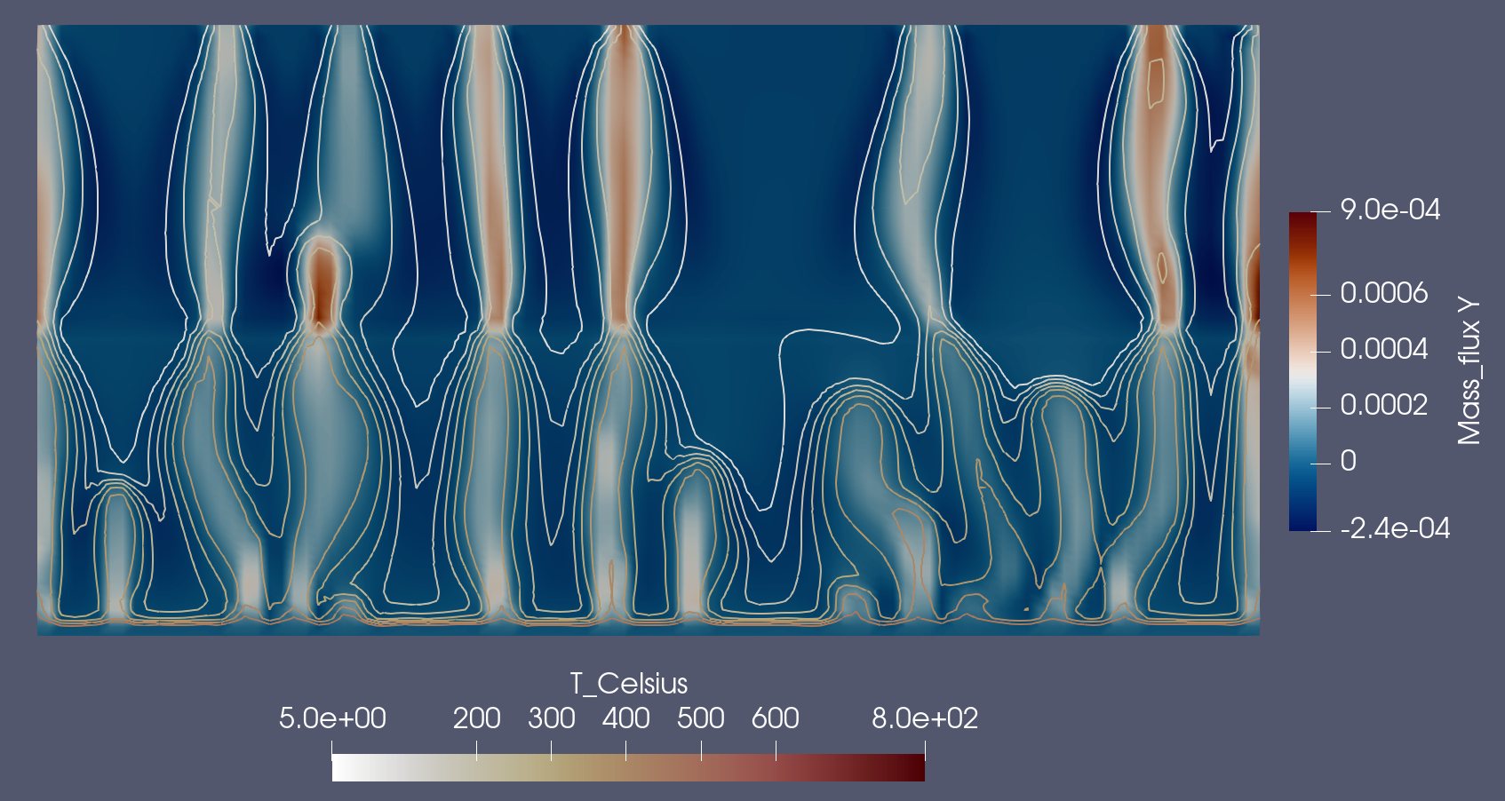
Puzzle temperature contours and vertical mass flux together and explore what happens at the interface.

../../_images/Flux_interface.png — Fig. 31 Vertical mass flux and temperature contours at the interface between the two layers.

Clearly, mass flux is increasing and temperature is decreasing. What do you think is happening to the convective heat flux?

We will now explore the interplay between permeability and bottom heat flux. The research question is: what kind of permeability is needed to sustain a high-temperature hydrothermal system? This question was addressed by [Driesner, 2010b].

Let’s first go through the theory. The flux into the reaction zone of hydrothermal convection cell can be written as:

(39)\[\vec{q_{in}} = 2\frac{L\lambda (T_D - T_U)}{H_R}\]

\(L\) is the half-width of the reaction zone, \(\lambda\) is the thermal conductivity, \(T_D\) the temperature of the driving heat source, \(T_U\) the upflow temperature, and \(H_R\) the thickness of the reaction zone.

Let’s follow [Jupp & Schultz, 2000] and explore the heat transported by hydrothermal convection. For this we have to make a few assumptions. The first is that the pressure gradient in the upwflow is close to cold hydrostatic \(\rho_0 g\), which is a reasonable assumption based on convection experiments.

Now we can use Darcy’s law to spell out the vertical velocity and mass flux:

(40)\[\vec{u} = -\frac{k}{\mu}( \nabla P - \rho \vec{g} )\]

(41)\[\frac{\partial P}{\partial z} = \rho_0 g_z\]

(42)\[u_z = -\frac{k}{\mu_U}g_z(\rho_0 - \rho_U)\]

(43)\[\rho_U u_z = -\frac{k}{\mu_U} \rho_U g_z(\rho_0 - \rho_U)\]

with \(_U\) always referring to properties within the upflow zone, which has a temperature of \(T_U\).

We can spell out the heat output by multiplying this with the difference in specific enthalpy \(h [J/Kg]\) between the upflow (\(h_U\)) and the recharge zone (\(h_0\)). To get the total heat flux, we also need to multiply with two times the half-width (\(L\)) of the upflow zone:

(44)\[2L\rho_U u_z (h_U - h_0) = 2gk \left[ \frac{\rho_U (h_U - h_0) (\rho_0 - \rho_U) }{\mu_U}\right]L\]

And by setting this equal to the heat input, we get:

(45)\[2\frac{L\lambda (T_D - T_U)}{H_R} = 2gk \left[ \frac{\rho_U (h_U - h_0) (\rho_0 - \rho_U) }{\mu_U}\right]L\]

Note how we “flipped” the sign of g for better readability and omitted the \(T_U\) index. If we replace the right-hand side with a given heat flux \(Q\) we get:

(46)\[Q = 2gk \left[ \frac{\rho_U (h_U - h_0) (\rho_0 - \rho_U) }{\mu_U}\right]L\]

Nice, we have an equation that relates heat input, permeability, and upflow temperature. Unfortunately, it is not that useful as the upflow temperature is hidden as an implicit term in the fluid properties.

Try it out!

Let’s implement the equation in python and explore the solution and implications. Go through the attached notebook, fill out the missing pieces and think about what this means for upflow temperatures in genetral and for heterogeneous rock in particular.

Upflow temperature as a function of permeability (Driesner 2010)

Numerical solution

Next we will explore this using our numerical model. A basic setup can be downloaded from here: Driesner2010.

The magma heat source is simulated by a heat flux boundary condition, which can be set by customized boundary condition type of hydrothermalHeatFlux (see doc ). The model in [Driesner, 2010b] is 1 m thick, 3 km wide, 1 km height, the heat source is simulated by a Gaussian-shaped heat flux profile with total heat input 86 kW/m, half-width 500 m and center 1500 m.

Let’s see how to set this boundary condition in HydrothermalFoam. hydrothermalHeatFlux supports Gaussian-shape (shape gaussian2d;) distribution and the shape is defined by four parameters x0, qmax, qmin, c, the equation of the shape is

(47)\[q_h(x) = q_{min} + (q_{max}-q_{min})e^{-\frac{(x-x_0)^2}{2c^2}}\]

for a normal Gaussian-shape profile in this model, qmin is set to zero and x0 is set to 1500. From equation equation (47), we can get the half-width and total heat flux (approximately) are \(c\sqrt{2ln2}\) and \((q_{max}-q_{min})\sqrt{2\pi}c\), respectively. According to the model setup, it’s easy to get \(c = \frac{500}{\sqrt{2ln2}} = 424.661\) and \(q_{max} = \frac{86}{c\sqrt{2\pi}} = 0.0808\ kW/m^2\). There the temperature boundary condition at the bottom patch can be set as,

Code snippet

Listing 25 Temperature boundary condition of bottom patch

bottom
{
    type        hydrothermalHeatFlux;
    q           uniform 0.05; //placeholder
    value       uniform 0; //placeholder
    shape       gaussian2d;
    x0          1500;
    qmax        80.8;
    qmin        0;
    c           424.661;
}

Heat flux profile

(Source code, svg, pdf)

Excercise

Set up a new run, for example with \(k=5e^{-14} m^2\), and compare the vent temperatures of the numerical simulation with the predictions of our semi-analytical solution.