FD calculation of radioactive decay

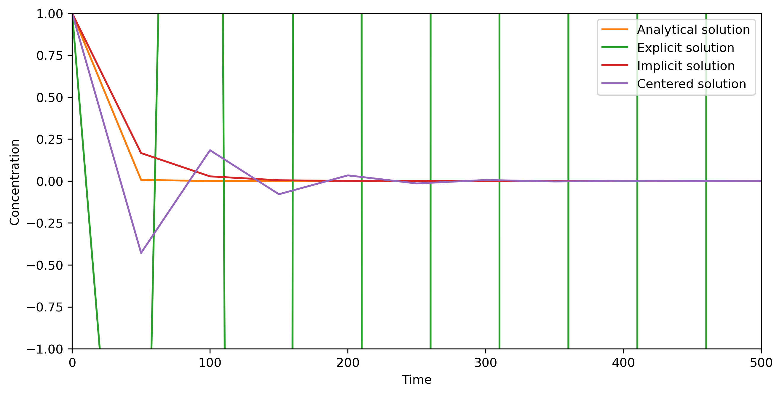
We will solve for radioactive using explicit and implicit FD schemes.

Load libraries and set resolution of output figures

import numpy as np
import matplotlib as mpl
import matplotlib.pyplot as plt
mpl.rcParams['figure.dpi']= 300

Define physics constants, here we use arbitrary values without any physical meaning

c0      = 1      # initial concentration
k       = 0.1    # decay constant

Setup numerics

dt      = 50                            # time step
steps   = 11                            # number of time steps
Cana    = np.zeros(steps)               # analytical solution
Cana[0] = c0                            # initial condition

Cexp    = Cana.copy()                   # make a copy
Cimp    = Cana.copy()
Ccen    = Cana.copy()

Time    = np.linspace(0, (steps-1)*dt, steps)  # time stepping, and Time vector

Perform calculation

# hide: the code in this cell is hidden by the author

# write update rules for the explicit and implicit cases!
# Bonus: write an update rule that uses the concentration at the middle of the time step
#for n in range(0,len(Cana)-1):

    # Cana[n+1] = np.exp(-k*Time[n+1])            #analytical
    # Cexp[n+1] = ???
    # Cimp[n+1] = ???

Plot different solutions

# First set up the figure, the axis, and the plot element we want to animate
fig = plt.figure(figsize=(10,5))
fig.clf()
ax  = plt.axes(xlim=(0, dt*(steps-1)), ylim=(-c0, c0))
line, = ax.plot([], [], lw=1)
ax.set_xlabel('Time')
ax.set_ylabel('Concentration')
plt.plot(Time, Cana, label='Analytical solution')
plt.plot(Time, Cexp, label='Explicit solution')
plt.plot(Time, Cimp, label='Implicit solution')
plt.plot(Time, Ccen, label='Centered solution')

plt.legend()

plt.show

<function matplotlib.pyplot.show(close=None, block=None)>