Example 2: Cooling dike - implicit version
In the previous session, we have learned how to solve for temperature using finite differences. However, our solution was only stable for certain parameter choices. In fact, we found that the finite differences formulation is only stable for \(\beta<0.5\):
Today we will explore how to formulate a finite differences model that is always stable.
Stability analysis
Before progressing let us explore when and why the explicit scheme is unstable. Let us assume a temperature profile with a single peak:
and let’s further assume that \(\beta = 0.2\). Then after one time step the temperature profile looks like this:
A nice diffusion profile. By further try-and-error (do it for different values for beta!), we find that the scheme is only stable for \(\beta<0.5\)
Radioactive decay analog
A good test problem to explore the stability and accuracy of different finite element schemes is radioactive decay. The change in concentration is controlled by this equation:
equation (36) states that the rate of decay is controlled by how much of the material is still there. To solve equation (36), we can use our standard finite differences approach:
This standard implementation is called the explicit form because you can write the new concentration directly as a function of the old one. The assumption here is that the concentration at the beginning of the time step controls the decay rate. An alternative formulation, the implicit form, is to assume that the decay rate is controlled by the (unknown) concentration at the end of the time step \(c^{n+1}\). The implicit from is therefore:
We will explore the differences between both formulations with a little python script.
FDM notebook
Excercise - radioactive decay
Try out the notebook and explore under which conditions the solutions are stable. What’s the difference between the explicit and the implicit solution?
Add another method to the script that takes the concentration at the center of the time step:
Implicit Heat Diffusion
The previous exercise on radioactive decay has shown that the fully implicit method is always stable. We will now rewrite our dike cooling model using the implicit formulation. Here is the implicit finite differences form:
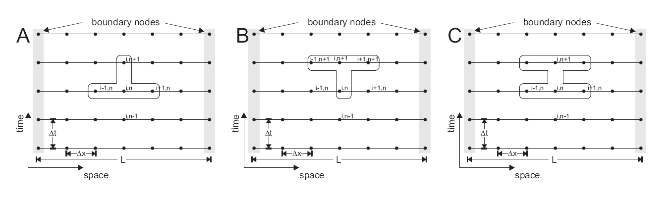
Fig. 3 Different explicit and implicit FD discretization stencils.
It is characteristic for the implicit form that the solution for \(T^{n+1}_i\) depends on the solution of the neighboring nodes (\(i-1\) and \(i+1\)). As a consequence, we cannot simply solve for one node after the other anymore but need to solve a system of equations. In fact, the way forward is to state the problem in matrix form \(A\vec{x}=\vec{b}\) and solve all equations simultaneously:
All we need to do is set up the matrix A and then solve for \(T^{n+1} = A \backslash T^n\)!
FDM notebook
Excercise - implicit dike cooling
Get the notebook to work and programm the implicit solution. Explore if you find any stability limits.
Bonus: Plot the explicit and implicit solutions together. Do you find the same behavior as in the radioactive decay example?