Triangles: unstructured meshes¶

In this session we will learn

how to use a mesh generator to mesh complex geometries,

what changes are needed to change the basic element.

The problem we will look at is basically the same as in the example given above. We will resolve steady-state heat diffusion within a rectangular region but now we will have circular inclusions of different thermal conductivity.

Theoretical background¶

Let’s first explore how triangle element “work”. Fig. 16 shows a triangle in global and local coordinates. The local node numering is again counterclockwise.

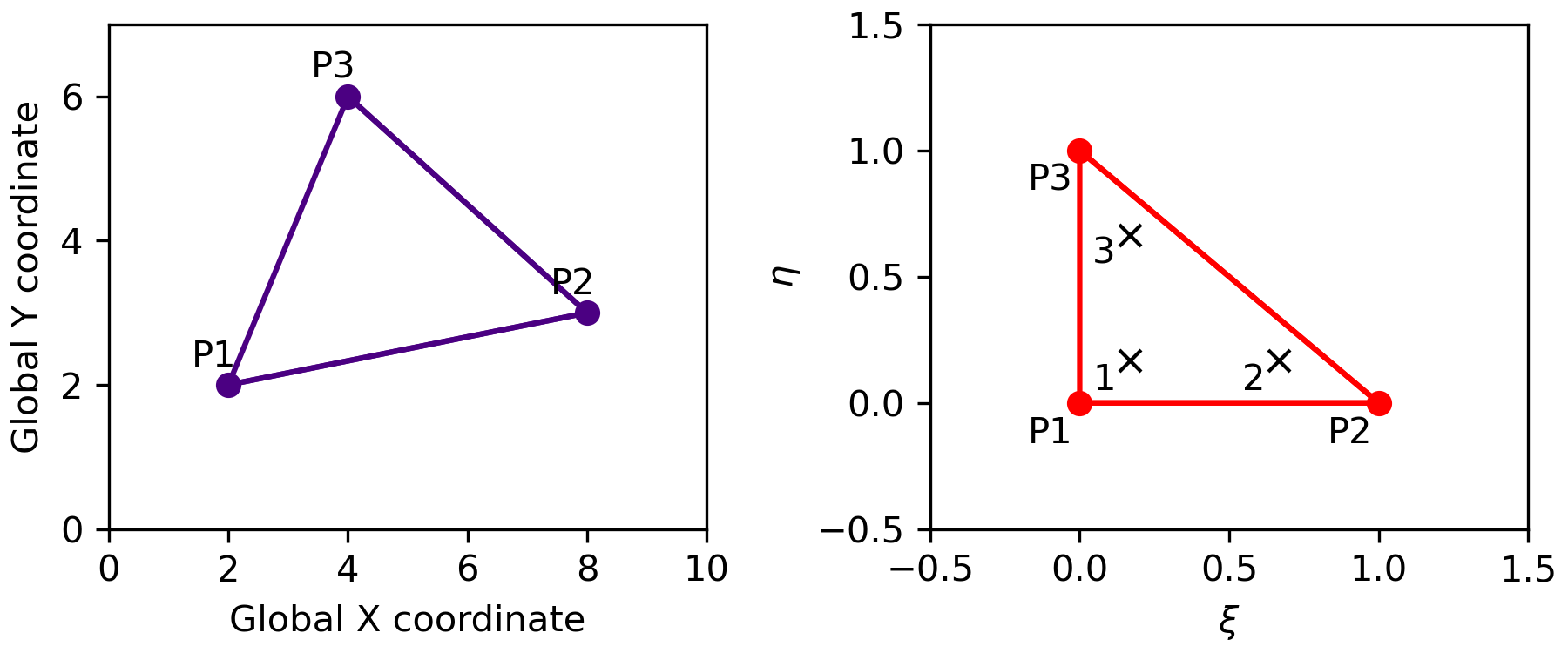
Fig. 16 Global and local coordinates of a triangle element. Black crosses mark the locations of the three integration points.¶

Here we look at a linear triangle with three nodes. The relation between global and local coordinates is therefore:

(135)¶\[\begin{split}\begin{align} \begin{split} x &= x_1 + (x_2-x_1)\xi + (x_3-x_1)\eta \\ y &= y_1 + (y_2-y_1)\xi + (y_3-y_1)\eta \\ \end{split} \end{align}\end{split}\]

Temperature, or any other variable, will also vary linearly with the local coordinates and we can write

(136)¶\[T(\xi,\eta) = a_1 +a_2\xi + a_3\eta\]

We can spell this out for the three nodes:

(137)¶\[\begin{split}\begin{align} \begin{split} T_1 &= T(0,0) = a_1 \\ T_2 &= T(1,0) = a_1 + a_2 \\ T_3 &= T(0,1) = a_1 + a_3 \end{split} \end{align}\end{split}\]

And express the contants \(a\) in terms of the nodal temperatures (or whatever our unknown is).

(138)¶\[\begin{split}\begin{align} \begin{split} a_1 = T_1 \\ a_2 = T_2 - T_1 \\ a_3 = T_3 - T_1 \end{split} \end{align}\end{split}\]

This we put back into the definition of the approximate solution equation (136) and get:

(139)¶\[\begin{split}\begin{align} \begin{split} T(\xi,\eta) &= T_1 +(T_2 - T_1)\xi + (T_3-T_1)\eta\\ \Rightarrow \\ T(\xi,\eta) &= (1 -\xi - \eta)T_1 + \xi T_2 + \eta T_3 \\ \Rightarrow \\ N_1(\xi, \eta) &= (1 -\xi - \eta)\\ N_2(\xi, \eta) &= \xi \\ N_3(\xi, \eta) &= \eta \\ \Rightarrow \\ T(\xi,\eta) &= N_1 T_1 + N_2 T_2 + N_3 T_3 \\ \end{split} \end{align}\end{split}\]

Alright, now that we understand the local coordinates and the shape functions associated with linear triangle element, we are good to go!

Excercise¶

Step 0: getting ready¶

Make a copy of the example solver above. Take it as a starting point and integrate the various code pieces and pieces of information below into.

Step 1: mesh generation¶

We will use the mesh generator triangle by Jonathan Shewchuk. It’s one of the best 2-D mesh generators for triangle meshes. It’s originally written in C but we will for convenience use a python wrapper. You can install it into your virtual environment by doing this:

pip install triangle

Here is a code piece for making the the mesh:

import triangle as tr

## Create the triangle mesh
vertices = []
segments = []
regions = []

# make a box with given dims and place given attribute at its center
def make_box(x, y, w, h, attribute):
    i = len(vertices)

    vertices.extend([[x,   y],
                    [x+w, y],
                    [x+w, y+h],
                    [x,   y+h]])

    segments.extend([(i+0, i+1),
                    (i+1, i+2),
                    (i+2, i+3),
                    (i+3, i+0)])

    regions.append([x+0.01*w, y+0.01*h, attribute,0.005])

def make_inclusion(center_x, center_y, radius, points_inc, attribute):
    theta        = np.linspace(0,2*np.pi,points_inc, endpoint=False)
    xx           = np.cos(theta)
    yy           = np.sin(theta)

    i = len(vertices)
    vertices.extend(np.array([center_x + radius*xx,center_y + radius*yy]).T)

    Tmp = np.array([np.arange(i, i+points_inc), np.arange(i+1, i+points_inc+1)]).T
    Tmp[-1,1] = i
    segments.extend(Tmp)

    regions.append([center_x, center_y, attribute,0.001])

#geometry
x0          = -1
y0          = -1
lx          = 2
ly          = 2
n_incl      = 5
radius      = 0.15

# generate input
make_box(x0, y0, lx, ly, 1)

make_inclusion(-0.8, -0.3, radius, 20, 100)
make_inclusion(-0.5, -0.75, radius, 20, 100)
make_inclusion(-0.6, 0.5, radius, 20, 100)
make_inclusion(-0.1, -0.3, radius, 20, 100)
make_inclusion(0.1, 0, radius, 20, 100)
make_inclusion(0.5, -0.2, radius, 20, 100)
make_inclusion(0.6, .3, radius, 20, 100)
make_inclusion(0.7, .8, radius, 20, 100)
make_inclusion(0, .75, radius, 20, 100)
make_inclusion(-0.5, .05, radius, 20, 100)
make_inclusion(0.5, -.75, radius, 20, 100)

A = dict(vertices=vertices, segments=segments, regions=regions)
B = tr.triangulate(A, 'pq33Aa')
#tr.compare(plt, A, B)
#plt.show()

# extract mesh information
GCOORD = B.get("vertices")
EL2NOD = B.get("triangles")
Phases = B.get("triangle_attributes")

nnodel = EL2NOD.shape[1]
nel    = EL2NOD.shape[0]
nnod   = GCOORD.shape[0]
Phases = np.reshape(Phases,nel)

Note how the generated mesh comes back as a python dictionary from which we extract the mesh information. Note also that the array Phases contains a marker to which region an element belongs (matrix versus inclusion).

Step 2: triangle shape functions and integration points¶

Fig. 5 shows shape functions for a linear triangle element. You will need to modify the function in our shapes.py file to implement the triangular shape functions.

#shape functions
eta2 = xi
eta3 = eta
eta1 = 1-eta2-eta3

N1 = eta1
N2 = eta2
N3 = eta3

Take this as a starting point and modify shapes.py to return the correct three shape functions and the six derivatives!

Next we need to adapt our integration rule. Take these three integration points and weights.

Table 2 Triangle integration¶
Integration point	\(\xi\)	\(\eta\)	weight
\(1\)	\(\frac{1}{6}\)	\(\frac{1}{6}\)	\(\frac{1}{6}\)
\(2\)	\(\frac{2}{3}\)	\(\frac{1}{6}\)	\(\frac{1}{6}\)
\(3\)	\(\frac{1}{6}\)	\(\frac{2}{3}\)	\(\frac{1}{6}\)

Tip

There are, of course, many different elements and associated integration rules using different numbers of integration points in FEM. Have a look at the suggested books in Course details .

Step 3: Boundary conditions¶

We were actually a bit “lazy” when we implemented the boundary conditions in the example above. Instead of coming up with a general solution, we identified the global node numbers on the boundaries assuming a structured quad mesh. Now we are using an unstructured triangle mesh and it is not so easy anymore to know which nodes are on the boundaries and should get boundary conditions. The “typical” way would be to use boundary markers in the mesh generation; here we use a different approach and use an ad-hoc search for the boundary nodes:

# indices and values at top and bottom
tol = 1e-3
# i_bot = np.where(abs(???) < tol)[0] #bottom nodes
# i_top = np.where(abs(???) < tol)[0] #top nodes

Complete this and add the lines to the main code!

Boundary conditions

Did you notice that we are not specifying boundary conditions for lateral boundaries? Still the code seems to work. Have a look at equation (119) and think about which implicit assumption we are making about the line integral.

Step 4: Post-processing and plotting¶

Modify the post-processing code that computes the heat fluxes, so that it works for triangles. This should just involve setting a new local coordinates for the single integration points. Use \(\xi=\frac{1}{3}\) and \(\eta=\frac{1}{3}\), which is the center of each triangle.

Now we just need to plot! Thankfully python makes it easy for us and we can use the functions triplot and tricontourf to plot the unstructured data.

# plotting
fig = plt.figure()
left, bottom, width, height = 0.1, 0.1, 0.8, 0.8
ax = fig.add_axes([left, bottom, width, height])

plt.triplot(GCOORD[:,0], GCOORD[:,1], EL2NOD, linewidth=0.5)
cp = plt.tricontourf(GCOORD[:,0], GCOORD[:,1], EL2NOD, T, 10, cmap='gist_yarg')

plt.colorbar(cp)
plt.quiver(Ec_x, Ec_y, Q_x, Q_y, np.sqrt(np.square(Q_x) + np.square(Q_y)), cmap='hot')

ax.set_title('Temperature with heat flow vectors')
ax.set_xlabel('x')
ax.set_ylabel('y')
plt.show()

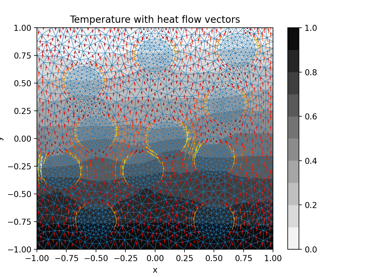
Fig. 17 2-D diffusion on unstructured mesh.¶