Introduction: The Finite Differences Method (FDM)
Before progressing towards finite element modeling, we will learn about the Finite Difference Method (FDM), which is a somewhat easier method to solve partial differential equations. We will do so by looking at how heat conduction “works”.
Background on conductive heat transport
Temperature is one of the key parameters that control and affect the geological processes that we are exploring during this class. Mantle melting, rock rheology, and metamorphism are all functions of temperature. It is therefore essential that we understand how rocks exchange heat and change their temperature.
One fundamental equation in the analysis of heat transfer is Fourier’s law for heat flow:
It states that heat flow is directed from high to low temperatures (that’s where the minus sign comes from) and is proportional to the geothermal gradient. The proportionality constant, k, is the thermal conductivity which has units of W/m/K and describes how well a rock transfers heat. k is a typically a complex function of rock type, porosity, and temperature yet is often simplified to a constant value.
In most cases, we are interested in temperature and not heat flow so that we would like to have an equation that describes the temperature evolution in a rock. We can get this by starting from the convervations equation of internal energy.
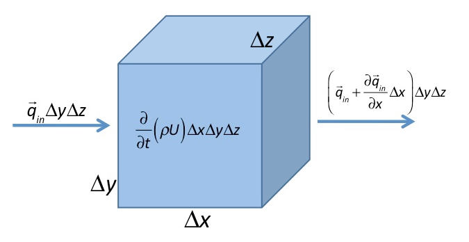
Fig. 1 Derivation of the energy equation. Change in internal energy is related to changes in heat fluxes into and out of the box (and a lot of other terms (e.g. advection) that are neglected here).
For simple incompressible cases, changes in internal energy can be expressed as changes in temperature times density and specific heat. The change in internal energy with time can now be written as \(\rho c_p \frac{\partial}{\partial t} T \Delta x \Delta y \Delta z\) (\(\rho\) is density, \(c_p\) specific heat, and \(T\) temperature), has units of (\(J/s\)), and must be equal to the difference between the heat flow into the box \(q_{in} \Delta y \Delta z \left( \frac{W}{m K}\frac{K}{m}m^2 = \frac{J}{s}\right)\) and the heat flow out of the box \(\left( q_{in} + \frac{\partial q_{in}}{\partial x} \Delta x\right) \Delta y \Delta z\) (the y and z directions are done in the same way). With these considerations, we can write a conservation equation for energy in 1D:
equation (2) is called the heat transfer or heat diffusion equation and is one of the most fundamental equations in Earth Sciences. If the thermal conductivity is constant, we can define a thermal diffusivity, \(\kappa\), and write the simpler second form of the equation.
Note that in 3D, the changes in heat flow are expressed as a divergence:
Or in vector notation:
Finite Differences discretization
equation (2) is a partial differential equation that describes the evolution of temperature. There are two fundamentally different ways to solve it: 1) analytically or 2) numerically. Analytical solutions have the virtue that they are exact but it is often not possible to find one for complex systems. Numerical solutions are always approximations but can be found also for very complex systems. We will first use one numerical technique called finite differences. To learn how partial differential equations are solved using finite differences, we have to go back to the definition of a derivative:
In our case, the above derivative describes the change in temperature with x (our space coordinate). In numerics, we always deal with discrete functions (as opposed to continuous functions), which only exist at grid points Fig. 2. We can therefore translate the above equation into computer readable form:
\(T(i)\) is the temperature at a grid point \(i\) and \(\Delta x\) is the grid spacing between two grid points. Using this definition of a derivative, we can now compute the heat flow from the calculated temperature solution:
This form is called the finite differences form and is a first step towards solving partial differential equations numerically.
Note that it matters in which direction you count. Usually it makes life much easier if indices and physical coordinates point in the same direction, e.g. x coordinate and index increase to the right.
We have learned how we can compute derivatives numerically. The next step is to solve the heat conduction equation (equation (2)) completely numerically. We are interested in the temperature evolution as a function of time and space \(T(x, t)\), which satisfies equation (2), given an initial temperature distribution. We know already from the heat flow example how to calculate first derivatives (forward differencing):
The index \(n\) corresponds to the time step and the index \(i\) to the grid point (x-coordinate, Fig. 2). Next, we need to know how to write second derivatives. A second derivative is just a derivative of a derivate. So we can write (central differencing):
If we combine equation equation (8) and equation (9) we get:
Tip
Notice how we have conveniently used the time index \(n\) for the temperatures in the spatial derivatives. This results in the explicit form of the final discretized equation. The implicit form, which we will learn about later, would used the unknown new (time index \(n+1\)) temperatures for the spatial derivatives, which requires solving a system of equations.
The last step is a rearrangement of the discretized equation, so that all known quantities (i.e. temperature at time \(n\)) are on the right-hand side and the unknown quantities on the left-hand side (properties at \(n+1\)). This results in:
We have now translated the heat conduction equation equation (2) into a computer readable finite differences form.
Appendix
Taylor-series expansions
Finite difference approximations can be derived through the use of Taylor-series expansions. Suppose we have a function \(f(x)\), which is continuous and differentiable over the range of interest. Let’s also assume we know the value \(f(x_0)\) and all the derivatives at \(x = x_0\). The forward Taylor-series expansion for \(f(x_0+\Delta x)\) about \(x_0\) gives
We can compute the first derivative by rearranging equation ref{eqs:Taylor_series_expansion}
This can also be written in discretized notation as:
here \(O(\Delta x)\) is called the truncation error, which means that if the distance \(\Delta x\) is made smaller and smaller, the (numerical approximation) error decreases with \(\Delta x\). This derivative is also called first order accurate.
We can also expand the Taylor series backward
In this case, the first (backward) derivative can be written as
By adding equation (13) and equation (16) and dividing by two, a second order accurate first order derivative is obtained
By adding equations equation (13) and equation (15) an approximation of the second derivative is obtained
With this approach we can basically derive all possible finite difference approximations. A different way to derive the second derivative is by computing the first derivative at \(i+\frac{1}{2}\) and at \(i-\frac{1}{2}\) and computing the second derivative at \(i\) by using those two first derivatives:
Similarly we can derive higher order derivatives. Note that the highest order derivative that usually occurs in geodynamics is the \(4^th\)-order derivative.
Finite difference approximations
The following equations are common finite difference approximations of derivatives. If you, in the future, need to write a finite difference approximation, come back here.
Left-sided first derivative, first order
Right-sided first derivative, first order
Central first derivative, second order
Central first derivative, fourth order
Central second derivative, second order
Central second derivative, fourth order
Central third derivative, second order
Central third derivative, fourth order
Central fourth derivative
Note that the higher the order of the finite difference scheme, the more adjacent points are required. It is also important to note that derivatives of the following form
should be formed as follows