Example 1: Cooling dike
Problem description
As a first example, we will use the finite differences form (equation (11)) of the heat diffusion equation (equation (2)) to explore the cooling of a dike. We will look at a \(2m\) wide dike that intruded with a temperature of \(1200°C\) into \(300°C\) warm country rock. The initial conditions can be written as:
In addition, we assume that the temperature far away from the dike center (at \(\lvert L/2 \rvert\)) remains at a constant temperature. The boundary conditions are thus:
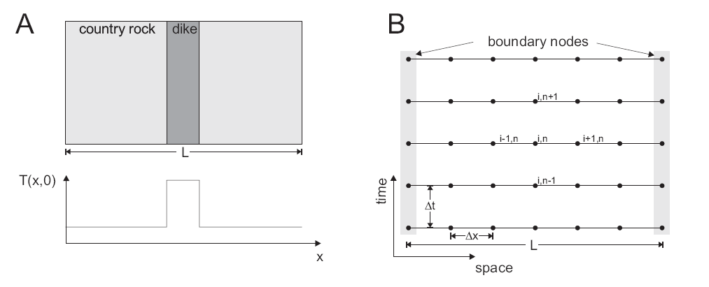
Fig. 2 summarizes the setup of the cooling dike problem.

Fig. 2 Setup of the model considered here (A). A hot basaltic dike intrudes into colder country rock. Only variations in x-direction are considered; properties in the other directions are assumed to be constant. The initial temperature distribution \(T(x,0)\) has a step-like perturbation. B) Finite difference discretization of the 1D heat equation. The finite difference method approximates the temperature at given grid points, with spacing \(\Delta x\). The time-evolution is also computed at given times with timestep \(\Delta t\).
Excercises - 1-D cooling dike (explicit)
Try to implement the above prolem in python using the juypter notebook below as a starting point. One way is to activate your course python environment, start a jupyter lab or notebook, and create a new notebook. You can then copy the code blocks (cells) from the script into your notebook and complete the missing pieces.
conda activate py37_fem_lecture
cd $your_working_directory$
jupyter lab
Now you can explore the numerical solution.
Complete the notebook and get it to work
Vary the parameters (e.g. use more gridpoints, a larger timestep). Notice how the numerical solution becomes unstable when the timestep is increased beyond a certain value. What does this value depend on? This is a major drawback of explicit finite difference codes such as the one presented here.
Record and plot the temperature evolution versus time at a distance of 5 meter from the dike/country rock contact. What is the maximum temperature the country rock experiences at this location and when is it reached?
Bonus question: Derive a finite-difference approximation for variable k and variable dx.
Here is a starting point for also calculating the temperature evolution at a certain distance from the dike.