Exercise 2

Now that we have simulated 2-D cavity flow, it is time to try 3-D flow and parallel processing.

3-D cavity flow

First, try to make a 3-D simulation. Start from a fresh copy of the original tutorial, not from your own cavity2D: you have probably changed the mesh, the viscosity, or the time step there, and a combination that worked in 2-D may not work in 3-D. Copy the two scripts from your 2-D case:

cd $HOME/HydrothermalFoam_runs
cp -r $FOAM_TUTORIALS/incompressible/icoFoam/cavity/cavity cavity3D
cp cavity2D/run.sh cavity2D/clean.sh cavity3D/
cd cavity3D

Now these things have to happen

• make the mesh 3-D: in system/blockMeshDict, use 20 cells in each direction, (20 20 20)

• make the domain a cube: the cavity is only 0.01 m thick so far. Change the z coordinate of the four vertices with z = 0.1 to 1, so that the cavity is 0.1 m deep (remember convertToMeters 0.1)

• the front and back sides must not be “empty” anymore. There are three places where you have to change this: the patch type in system/blockMeshDict, and the boundary conditions in 0/U and 0/p

• set proper boundary conditions for front and back: they are walls now, just like the fixed walls. Which conditions do the fixed walls have in 0/U and 0/p?

• keep the time settings of the tutorial in system/controlDict: deltaT 0.005, endTime 0.5, writeInterval 20 (results every 0.1 s)

• run ./run.sh, check the Courant number in log.icoFoam, and inspect the results in ParaView

With these settings, the maximum Courant number is about 0.85, and the run takes only a few seconds.

Tip

If something goes wrong, read the error message carefully, it usually names the file and the patch with the problem. A frequent error is a patch that is empty in one file but not in the others.

Warning

A finer mesh needs a smaller time step. With 40 cells in each direction, the cells are half as large, so deltaT must be halved as well: use deltaT 0.0025 and writeInterval 40. The run then takes about half a minute. If you keep deltaT 0.005, the Courant number is about 2, the solution grows until it becomes nan (“not a number”) after about 0.2 s, and the results are useless. Depending on your computer, the run then either stops with a Floating point exception, or it continues to the end without an error message, so always check Courant Number in the log.

Getting fancy - let’s make a parallel run

Three-dimensional simulations can need substantial computing resources. OpenFOAM can distribute the work across several processor cores. The standard parallelization technique in OpenFOAM is called “domain decomposition”. This means that the computational domain is split into sub-domains and each subdomain is handled by a separate process, usually running on its own processor core. As always, all of this is controlled via a dictionary file. This file is called system/decomposeParDict .

To get started we make a copy of our 3-D case.

cd $HOME/HydrothermalFoam_runs
cp -r cavity3D cavity3D_par
cd cavity3D_par
./clean.sh

Unfortunately, there is no file system/decomposeParDict in our example case… Fortunately, there is probably an example file somewhere in all the provided tutorials. A simple way to find and copy one is this:

find  $FOAM_TUTORIALS -name "decomposeParDict"
...
/opt/OpenFOAM-10/tutorials/heatTransfer/chtMultiRegionFoam/heatedDuct/system/decomposeParDict
/opt/OpenFOAM-10/tutorials/heatTransfer/buoyantFoam/externalCoupledCavity/system/decomposeParDict
/opt/OpenFOAM-10/tutorials/heatTransfer/buoyantFoam/iglooWithFridges/system/decomposeParDict
...
cp /opt/OpenFOAM-10/tutorials/heatTransfer/buoyantFoam/iglooWithFridges/system/decomposeParDict $HOME/HydrothermalFoam_runs/cavity3D_par/system

Now open this file and edit it. The tutorial file is set up for two subdomains; change it to four subdomains and to the method simple, so that it looks like this (the other coefficient blocks in the file are not used and you can delete them):

Listing 12 Domain decomposition and parallel processing.

/*--------------------------------*- C++ -*----------------------------------*\
  =========                 |
  \\      /  F ield         | OpenFOAM: The Open Source CFD Toolbox
   \\    /   O peration     | Website:  https://openfoam.org
    \\  /    A nd           | Version:  10
     \\/     M anipulation  |
\*---------------------------------------------------------------------------*/
FoamFile
{
    format      ascii;
    class       dictionary;
    object      decomposeParDict;
}
// * * * * * * * * * * * * * * * * * * * * * * * * * * * * * * * * * * * * * //

numberOfSubdomains 4;

method          simple;

simpleCoeffs
{
    n               (2 2 1);
}

// ************************************************************************* //

With the method simple, our uniform rectangular domain is split into equally sized blocks: n (2 2 1) means two blocks in the x direction, two in the y direction, and one in the z direction. The product of the three numbers must equal numberOfSubdomains. Other methods, e.g. scotch, split the domain automatically and do not use simpleCoeffs. Details can be found in the OpenFOAM User Guide.

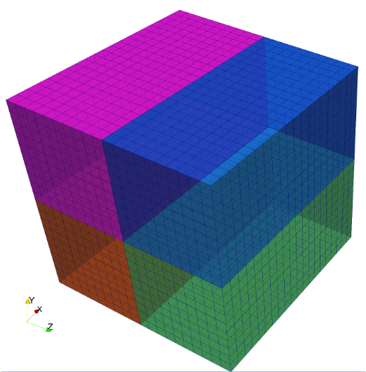
Fig. 10 A 3-D cavity mesh decomposed into four subdomains. Each colour is the part of the mesh that one processor works on.

Next you need to modify the run.sh script to invoke a parallel run.

cp run.sh run_par.sh

It should look like this:

Listing 13 The run_par.sh file.

#!/bin/sh
cd ${0%/*} || exit 1    # Run from this directory

# Source tutorial run functions
. $WM_PROJECT_DIR/bin/tools/RunFunctions

application=`getApplication`

./clean.sh
runApplication blockMesh
runApplication decomposePar
runParallel $application
reconstructPar

Run the parallel script in the container:

./run_par.sh

The runParallel function uses numberOfSubdomains to launch the solver. Make sure Docker has at least four CPU cores available for this example. The final reconstructPar command combines the results from the processor directories so that you can open a.foam in ParaView as before.

Compare the results and the run time (ExecutionTime at the end of log.icoFoam) with the serial run. With 20 × 20 × 20 cells, both runs take only about a second, so you will hardly notice a difference. The benefit becomes clear for larger meshes: in our test, a version with 60 × 60 × 60 cells (and a correspondingly smaller time step) took about 150 s on one core, 80 s on two, and 43 s on four cores. Note that the speedup is good, but less than the number of cores. The flow should look like this:

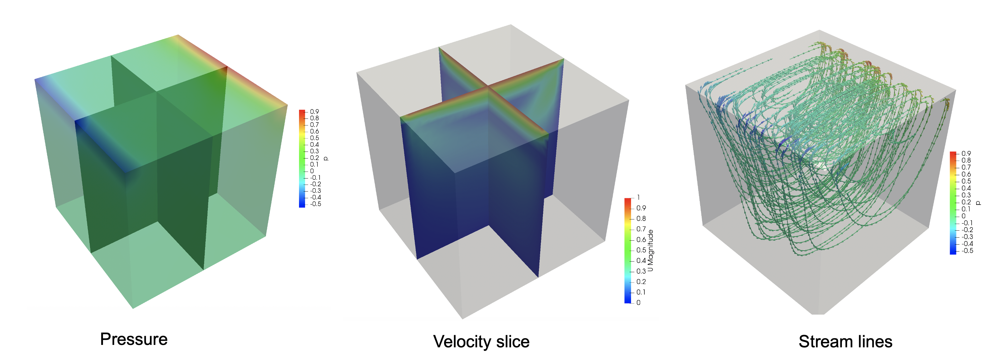
Fig. 11 Results of the 3-D parallel cavity flow simulation.