Python implementation
We will use our previously developed 2d FEM code for steady-state diffusion as a starting point and modify it to solve for Stokes flow. The implementation follows a dataclass-based architecture for better type safety and code organization, using containers for mesh data, material properties, boundary conditions, and solver parameters.
There are a number of extra complications in the Stokes flow problem that we need to address:
Data structures
The implementation uses dataclasses to organize code and data:
from dataclasses import dataclass

@dataclass
class Mesh:
    """Container for mesh data."""
    GCOORD: np.ndarray   # Node coordinates
    EL2NOD: np.ndarray   # Element connectivity
    Phases: np.ndarray   # Phase/material ID per element
    Node_ids: np.ndarray # Node boundary markers
    nnod: int = 0
    nel: int = 0
    nnodel: int = 0

@dataclass
class MaterialParams:
    """Container for material properties."""
    Mu: np.ndarray   # Shear viscosity per phase
    Rho: np.ndarray  # Density per phase
    G: np.ndarray    # Gravity vector [gx, gy]
Global degrees of freedom
In the steady-state diffusion problem, we had one degree of freedom per node. In the Stokes flow problem, we have two degrees of freedom per node: one for the x-velocity and one for the y-velocity. We will therefor have to double the number of degrees of freedom in the global stiffness matrix and the global force vector. We use a numbering where the 0th node has the degree of freedom 0 (x-velocity) and the degree of freedom 1 (y-velocity), the 1st node has the degrees of freedom 2 and 3, and so on. We will have to modify the code to account for this new numbering.
# BUILD ELEMENT-TO-DOF MAPPING
EL2DOF = np.zeros((nel, nedof), dtype=np.int32)
EL2DOF[:, 0::ndim] = ndim * mesh.EL2NOD
EL2DOF[:, 1::ndim] = ndim * mesh.EL2NOD + 1
We will use this matrix \(EL2DOF\) to construct the global stiffness matrix and the global force vector.
Pressure shape functions
Step one is to spell out what the pressure shape functions are. In our derivation, we just stated that pressure is discontinuous and varies linearly over the element. We therefor have three unknown pressures per element. But what are those shape functions?
We start with the assumption that pressure varies linearly as a function of global x,y coordinates.
Where \(a\),:math:b,:math:c are coefficients to be determined. The simplest linear shape function for a triangle with vertices at \((x_1,y_1)\), \((x_2,y_2)\), \((x_3,y_3)\) can be defined using barycentric coordinates or directly in terms of x and y coordinates.
We will find those shape functions by solving a linear system of equations. Let’s define a matrix \(P\) and a vector \(Pb\) as follows:
and a vector \(Pb\) as follows:
where \(x\) and \(y\) are the coordinates of an integration point (or any point in the element). The interpolation functions (or shape functions) can now be found for solving the following linear system of equations:
And we can find the shape functions as follows:
In the python FEM implementation, we will spell out the matrix \(P\) and the vector \(Pb\) using the coordinates of the vertices of the element and the coordinates of the integration point; solving the matrix equation above will give us the pressure shape functions.
# np_edof is the number of pressure degrees of freedom (here 3)
# ECOORD_X is a 7x2 matrix holding the x and y coordinates of the element vertices
ECOORD_X = mesh.GCOORD[mesh.EL2NOD[iel, :], :]
P = np.ones((np_edof, np_edof))
P[1:3, :] = ECOORD_X[:3].T
Inside the integration loop, we construct \(Pb\) and solve for the pressure shape functions:
for ip in range(solver.nip):
    # Ni is [7,] and holds the velocity shape functions
    # Ni @ ECOORD_X is then [2,] and holds the x and y coordinates of the integration point
    # Pi is [3,] and holds the pressure shape functions

    Pb[1:3] = Ni @ ECOORD_X
    Pi = np.linalg.solve(P, Pb)
Assembly of global matrices and pressure numbering
Finally, we need to assemble the global matrices. This includes the global \(Q\) and \(invM\) matrices, which we will use to reconstruct pressure from the velocity solution eq:pressure_static_condensation .
As the pressure is discontinuous, each element has three independent pressure unknowns. The numbering is therefore that element 0 has unknown pressures 0,1,2 and element 1 has unknown pressures 3,4,5, and so on. For the global \(Q\) matrix, the rows (i index) are therefore given by this continuous pressure numbering and the columns (j-index) by the matrix \(EL2DOF\).
# Build global Q matrix for discontinuous pressure
# element[0] -> pressure = [0,1,2]
# element[1] -> pressure = [3,4,5]
# The velocity dofs come from EL2DOF

Q_i = np.tile(np.arange(0, nel*np_edof, dtype=np.int32), (nedof, 1)).T
Q_j = np.tile(EL2DOF, (1, np_edof))
Q_all = csr_matrix((Q_all.ravel(), (Q_i.ravel(), Q_j.ravel())),
                   shape=(nel*np_edof, sdof))
The assembly of the global \(invM\) matrix is similar. The rows and columns are both given by the continuous pressure numbering.
invM_i = np.tile(np.arange(0, nel*np_edof, dtype=np.int32), (np_edof, 1)).T
base_sequence = np.tile(np.arange(np_edof), nel * np_edof)
offsets = np.repeat(np.arange(nel) * np_edof, np_edof**2)
column_indices = base_sequence + offsets
invM_all = csr_matrix((invM_all.ravel(), (invM_i.ravel(), column_indices.ravel())),
                      shape=(nel*np_edof, nel*np_edof))
The solver function signature follows the dataclass pattern:
def solve_mechanical_2d(
    mesh: Mesh,
    material: MaterialParams,
    bc: BoundaryConditions,
    solver: SolverParams
) -> Solution:
    """
    Solve 2D incompressible Stokes flow using FEM.

    Returns Solution object with velocity and pressure fields.
    """
There might be a more elegant solution to this; we’d be happy to hear about it!
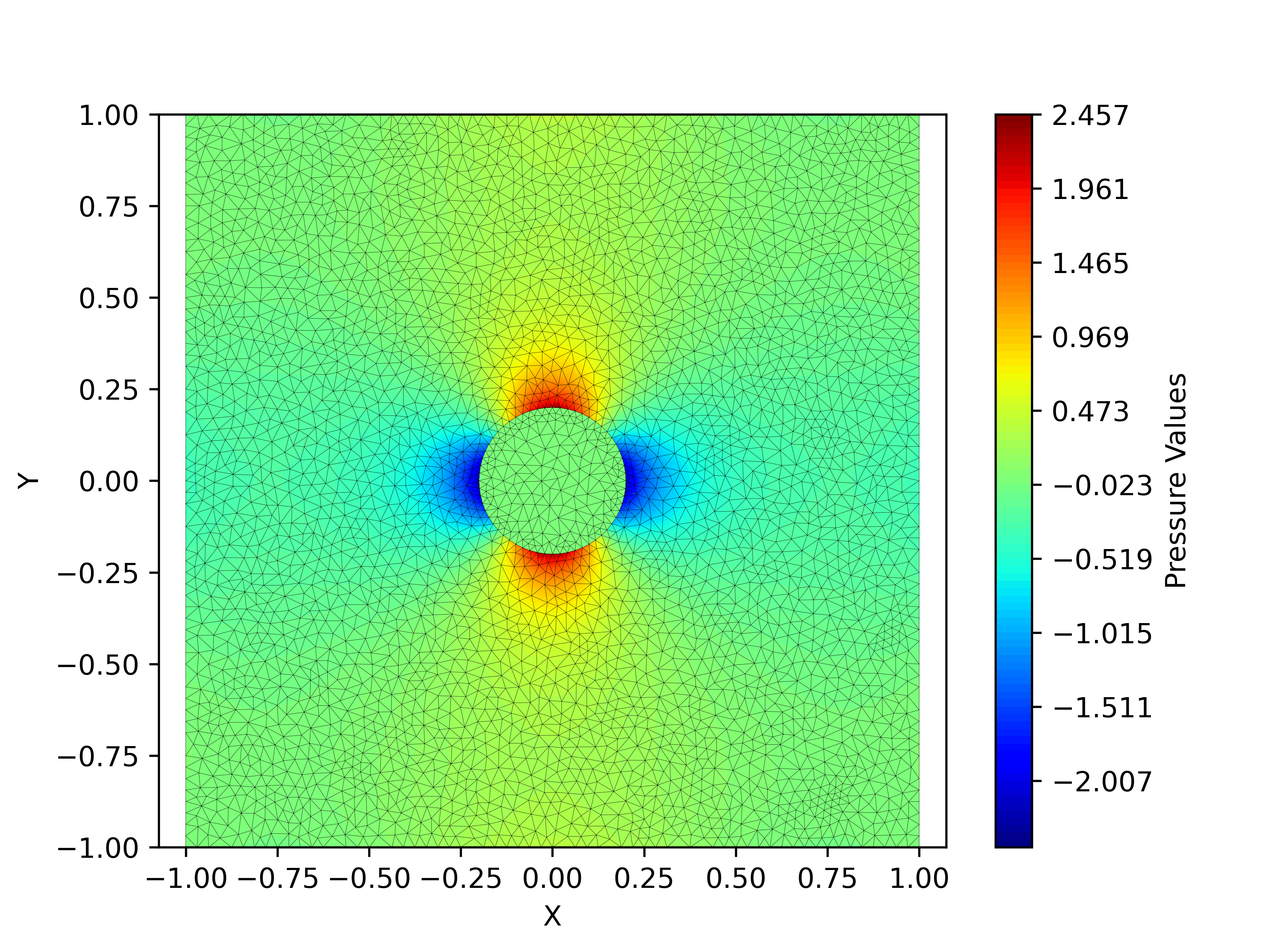
Test problem
We will use a test problem from structural geology to test our implementation. The problem is a pure shear problem with velocity boundary conditions at the sides and one (or multiple) inclusions of variable viscosity inside the modeling domain. Depending on the viscosity contrast, these inclusions will result in pressure anomalies. The problem has been explored analytically in [Schmid & Podladchikov, 2003].
You can download the code for this lecture here: ip_triangle.py, shp_deriv_triangle.py, mechanical2d_driver.py, and mechanical2d.py.
Exercises
Get the code to work and try to solve the following exercises:
Modify the
MaterialParamsto solve for a different problem, e.g., the pure shear problem with inclusions of different viscosity contrast.Modify the
make_mesh()function to create inclusions of different shapes (elliptical, rectangular, etc.).Modify the code to resolve inclusions of different density. This involves changing the boundary conditions to no-slip and adding gravity to
MaterialParams.G. If you want, add a pseudo time loop in whichmesh.GCOORDis updated using the computed velocities. This will give you a time-dependent problem with a moving inclusion.