Introduction to Stokes flow

The Stokes equation describes the flow of a viscous fluid in a slow regime. It is a simplification of the Navier-Stokes equation, which describes the flow of a fluid in a fast regime. The Navier-Stokes equation is a non-linear partial differential equation and is difficult to solve. The Stokes equation is a linear partial differential equation and is easier to solve. The Stokes equation is often used in geodynamics to describe the flow of the Earth’s mantle.

It’s derivation can be done based on conservation laws for mass and momentum.

Conservation of Mass

Conservation of mass means that the amount of mass in our model space is always constant; no mass is created or destroyed. Mass \(m\) is directly related to density \(\rho\) by unit volume, and a change in mass will result in an equivalent change in density. The change in density in our model box is equal to the sum of the mass flux through all boundaries:

(152)\[\frac{\partial \rho}{\partial t} + \nabla \cdot (\rho v) = 0\]

This describes the change of density in a fixed observation cell due to the in- and outflux of mass. Such a fixed node is called an Euler node and is formulated from the node’s point of view.

Using Leibniz’s Law (\(\frac{\partial}{\partial x} \left(u v\right) = \frac{\partial u}{\partial x} v + \frac{\partial v}{\partial x} u\)), the continuity equation can be extended:

(153)\[\frac{\partial \rho}{\partial t} + \nabla \cdot (\rho v) = \frac{\partial \rho}{\partial t} + \rho \nabla \cdot v + v \cdot \nabla \rho = 0\]

One term (\(v \cdot \nabla \rho\)) is the dot product of the velocity vector \(v\) with the density gradient \(\nabla \rho\), representing the rate at which density changes as material flows along the velocity field. In 3D, this is \(v_x \frac{\partial \rho}{\partial x} + v_y \frac{\partial \rho}{\partial y} + v_z \frac{\partial \rho}{\partial z}\). This term describes Advection or Advective transport - the transport of density variations by the flow. The other term (\(\rho \nabla \cdot v\)) describes the change of density in the observational volume due to mass flux of constant density but varying velocity (compression or expansion).

For the case of constant density, it follows that \(\frac{\partial \rho}{\partial t}=0\), \(\nabla \rho=0\) and \(\frac{D \rho}{D t}=0\). This assumption is valid for incompressible material and is often used in geodynamics. The incompressible continuity equation in 2D looks like:

(154)\[\nabla \cdot v = \frac{\partial v_x}{\partial x} + \frac{\partial v_y}{\partial y} = 0\]

and describes the conservation of mass in an incompressible material.

Conservation of Momentum

Stress

Stress \(\sigma\) is the force acting on the side of a body. In a 2D square, we can have a force acting in the x-direction on both sides perpendicular to x: \(\sigma_{xx}\). A second force \(\sigma_{yy}\) acts in the y-direction on the sides perpendicular to y. These forces can be understood as ‘pulling’ in both x- and y-directions.

In addition, forces in the x-direction can also act on the sides parallel to x: shear stress \(\sigma_{xy}\). A second shear stress acts in the y-direction on the sides parallel to y: \(\sigma_{yx}\).

To describe all these forces acting on a body with only one name, we will need a tensor. In 2D, the stress tensor has the following form:

\[\begin{split}\sigma_{ij} = \begin{pmatrix} \sigma_{xx} & \sigma_{xy}\\ \sigma_{yx} & \sigma_{yy} \end{pmatrix}\end{split}\]

In the absence of internal forces, the angular momentum has to be conserved. This means that shear stresses can only act on our body if they won’t create a rotational component. This can only be achieved if the following condition is fulfilled: \(\sigma_{ij}=\sigma_{ji}\).

The mean of all acting perpendicular stresses defines the pressure in our body. The minus sign appears because stresses are designed as pulling forces, while pressure is the force pushing into the body.

(155)\[P = -(\sigma_{xx}+\sigma_{yy}+\sigma_{zz})/3\]

No shear forces are acting on a fluid at rest. The forces perpendicular to the body define the hydrostatic pressure. In addition, we can now define the deviatoric stress \(\sigma'_{ij}\), which denotes the deviation in the stress state from hydrostatic pressure.

(156)\[\begin{split}\begin{split} \sigma'_{ij} = \sigma_{ij} - (-P) = \sigma_{ij} + \delta_{i,j} P\\ \begin{pmatrix} \sigma'_{xx} & \sigma'_{xy}\\ \sigma'_{xy} & \sigma'_{yy} \end{pmatrix} = \begin{pmatrix} \sigma_{xx} & \sigma_{xy}\\ \sigma_{xy} & \sigma_{yy} \end{pmatrix} + \begin{pmatrix} P & 0\\ 0 & P \end{pmatrix} \end{split}\end{split}\]

where \(\delta_{i,j} P\) denotes the hydrostatic pressure (making use of the Kronecker delta \(\delta_{ij}\) where \(\delta_{i,j}=1\) for \(i=j\) and \(\delta_{ij}=0\) for \(i\neq j\), this selects the main diagonal of a matrix) and \(\sigma'_{ij}\) is the deviatoric stress component. This means that:

\[\sigma_{xy} = \sigma_{yx} = \sigma'_{xy} = \sigma'_{yx}\]

Strain and strain rate

Strain describes the actual deformation of a body due to stress acting on it. Strain is also described as a tensor with components acting perpendicular to the x- and y-directions, and shear components acting parallel to the direction of deformation.

\[\begin{split}\begin{split} \epsilon_{ij} = \begin{pmatrix} \epsilon_{xx} & \epsilon_{xy}\\ \epsilon_{yx} & \epsilon_{yy} \end{pmatrix} \end{split}\end{split}\]

where \(\epsilon_{ij}\) denotes the change of material displacement \(u_x, u_y\), i.e., deformation.

The deformation in each direction and all sides is denoted by the mean of the two deformations working opposite each other:

\[\begin{split} \epsilon_{ij} = \frac{1}{2} \left(\frac{\partial u_i}{\partial x_j} + \frac{\partial u_j}{\partial x_i}\right) \end{split}\]

\[\begin{split}\begin{split} \epsilon_{xx} &= \frac{1}{2} \left(\frac{\partial u_x}{\partial x} + \frac{\partial u_x}{\partial x}\right) = \frac{\partial u_x}{\partial x}\\ \epsilon_{xy} &= \frac{1}{2} \left(\frac{\partial u_x}{\partial y} + \frac{\partial u_y}{\partial x}\right) = \epsilon_{yx}\\ \epsilon_{yx} &= \frac{1}{2} \left(\frac{\partial u_y}{\partial x} + \frac{\partial u_x}{\partial y}\right) = \epsilon_{xy}\\ \epsilon_{yy} &= \frac{1}{2} \left(\frac{\partial u_y}{\partial y} + \frac{\partial u_y}{\partial y}\right) = \frac{\partial u_y}{\partial y}\\ \end{split}\end{split}\]

In fluids, and therefore in most convection problems in geodynamics, a constitutive relationship between stress and strain rate is used and the equations are formulated as the rate of change in material displacement or the strain rate \(\dot{\epsilon}_{ij}\), which is the change of strain \(\epsilon_{ij}\) in time. For a displacement velocity \(v_i = \frac{D u_i}{D t}\), the strain rate can be expressed as:

(157)\[\begin{split}\begin{split} \dot{\epsilon}_{ij} &= \frac{1}{2} \left(\frac{\partial v_i}{\partial x_j} + \frac{\partial v_j}{\partial x_i}\right)\\ \begin{pmatrix} \dot{\epsilon}_{xx} & \dot{\epsilon}_{xy}\\ \dot{\epsilon}_{yx} & \dot{\epsilon}_{yy} \end{pmatrix} &= \begin{pmatrix} \frac{\partial v_x}{\partial x} & \frac{1}{2} \left(\frac{\partial v_y}{\partial x} + \frac{\partial v_x}{\partial y}\right)\\ \frac{1}{2} \left(\frac{\partial v_x}{\partial y} + \frac{\partial v_y}{\partial x}\right) & \frac{\partial v_y}{\partial y} \end{pmatrix} \end{split}\end{split}\]

From this formulation, we can immediately recognize that \(\dot{\epsilon}_{xy}=\dot{\epsilon}_{yx}\).

Similar to the stress tensor, one can define a deviatoric strain rate tensor \(\dot{\epsilon}'_{ij}\) which describes the deviation from strain rate \(\dot{\epsilon}_{ij}\) due to net rotational forces or rigid body rotation. No shear strain rate acts on a rigid body (\(\dot{\epsilon}'_{xy}=\dot{\epsilon}'_{yx}=0\)), and the divergence of such a body is described as \(\nabla \cdot v = \dot{\epsilon}'_{xx} + \dot{\epsilon}'_{yy} = \dot{\epsilon}'_{kk}\).

(158)\[\begin{split}\begin{split} \dot{\epsilon}'_{ij} &= \dot{\epsilon}_{ij} - \delta_{ij} \frac{1}{3} \dot{\epsilon}_{kk}\\ \begin{pmatrix} \dot{\epsilon}'_{xx} & \dot{\epsilon}'_{xy}\\ \dot{\epsilon}'_{xy} & \dot{\epsilon}'_{yy} \end{pmatrix} &= \begin{pmatrix} \dot{\epsilon}_{xx} & \dot{\epsilon}_{xy}\\ \dot{\epsilon}_{xy} & \dot{\epsilon}_{yy} \end{pmatrix} + \begin{pmatrix} -\frac{1}{3} \dot{\epsilon}_{kk} & 0\\ 0 & -\frac{1}{3} \dot{\epsilon}_{kk} \end{pmatrix} \end{split}\end{split}\]

Stress balance

According to Newton’s second law of motion:

\[f = m a\]

the net force acting on a body is equal to its mass times its acceleration or change of velocity. To apply this in the x-direction, we will need to gather all forces acting on the body in the x-direction. We consider a 2D control volume of size \(\Delta x \times \Delta y\) with unit thickness in z; the index 1 denotes the face on the negative side (left/bottom) and 2 the face on the positive side (right/top).

(159)\[f_{x} = f_{xx1} + f_{xx2} + f_{xy1} + f_{xy2} + m g_x = m a_x\]

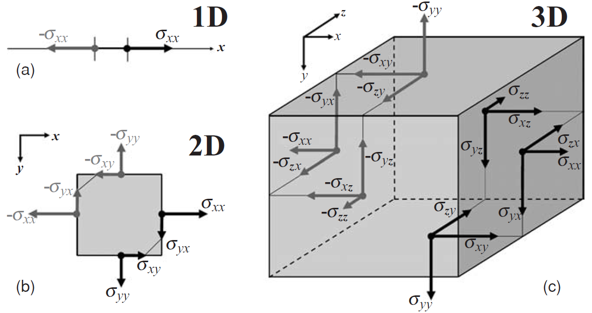
Fig. 19 Stresses acting on a 2D test volume (shown in 3D for clarity; unit thickness in z).

The forces can be described in terms of stresses:

\[\begin{split}\begin{split} f_{xx1} = -\sigma_{xx1}\Delta y\\ f_{xx2} = \sigma_{xx2} \Delta y\\ f_{xy1} = -\sigma_{xy1}\Delta x\\ f_{xy2} = \sigma_{xy2}\Delta x\\ \left(\sigma_{xx2} - \sigma_{xx1}\right)\Delta y + \left(\sigma_{xy2} - \sigma_{xy1}\right) \Delta x + m g_x = m a_x \end{split}\end{split}\]

Dividing equation equation (159) by the area of our 2D test volume \(A= \Delta x \Delta y\) (per unit thickness in z) then gives us:

\[\begin{split}\begin{split} \frac{\left(\sigma_{xx2} - \sigma_{xx1}\right)}{\Delta x} + \frac{\left(\sigma_{xy2} - \sigma_{xy1}\right)}{\Delta y} + \rho g_x = \rho a_x\\ \frac{\partial \sigma_{xj}}{\partial x_j} + \rho g_x = \rho \frac{D v_x}{D t}\qquad (j \in \{x,y\}) \end{split}\end{split}\]

Or in a more general form for all directions:

\[\begin{split} \frac{\partial \sigma_{ij}}{\partial x_j} + \rho g_i = \rho \frac{D v_i}{D t} \end{split}\]

By making use of equation equation (156) for the deviatoric stress, we arrive at the Navier-Stokes equation, which describes the conservation of momentum:

(160)\[\frac{\partial \sigma_{ij}'}{\partial x_j} - \frac{\partial P}{\partial x_i} + \rho g_i = \rho \frac{D v_i}{D t}\]

This equation makes use of the Einstein notation or Einstein summation convention. If an index appears twice in one term, this term actually stands for the sum of all possible values for this index. For example, the first term in the above equation equation (160) in 2D formulated in x actually hides the following:

\[\frac{\partial \sigma_{ij}'}{\partial x_j} = \frac{\partial \sigma_{xx}'}{\partial x} + \frac{\partial \sigma_{xy}'}{\partial y}\]

So the full Navier-Stokes equation in 2D actually has more terms and is a system of equations:

\[\begin{split}\begin{split} \frac{\partial \sigma_{xx}'}{\partial x} + \frac{\partial \sigma_{xy}'}{\partial y} - \frac{\partial P}{\partial x} + \rho g_x = \rho \frac{D v_x}{D t}\\ \frac{\partial \sigma_{yx}'}{\partial x} + \frac{\partial \sigma_{yy}'}{\partial y} - \frac{\partial P}{\partial y} + \rho g_y = \rho \frac{D v_y}{D t} \end{split}\end{split}\]

The term \(\rho \frac{D v_i}{D t}\) describes inertia and can be neglected in most geodynamic applications as it is much smaller than the gravitational acceleration. For a typical plate velocity of several \(\mathrm{cm/yr} \, (\sim 10^{-9} \mathrm{m/s})\) and a typical time for change in mantle flow of a few million years (\(\sim 10^{13} \mathrm{s}\)), inertia is of the magnitude of \(\sim 10^{-22} \mathrm{m/s^2}\). Compared to gravitational acceleration (\(\sim 10 \mathrm{m/s^2}\)), inertia is by a magnitude of \(\sim 10^{-23}\) smaller and can be safely neglected.

The resulting equation:

(161)\[\frac{\partial \sigma_{ij}'}{\partial x_j} - \frac{\partial P}{\partial x_i} + \rho g_i = 0\]

is called the Stokes equation of slow flow.

Stress-strain rate relationships

In elasticity, the stress is related to the strain by the Hooke’s Law: \(\sigma = C \epsilon\), where \(C\) is the stiffness tensor.

In viscous materials, the stress-strain rate relationship is typically written in terms of deviatoric stresses, deviatoric strain rates, and the shear viscosity \(\eta\). The shear viscosity is a measure of the resistance of a fluid to flow. The shear viscosity is a scalar in isotropic materials and a tensor in anisotropic materials.

The relationship between deviatoric stress and strain rates can be written as:

(162)\[\sigma_{ij}' = 2 \eta \dot{\epsilon}_{ij}'\]

The factor of 2 is introduced from the way the strain rate tensor is symmetrized in equation (157).

As our goal is to solve for the velocity field, we write the deviatoric strain rates as full strain rates using equation (158).

(163)\[\sigma_{ij}' = 2 \eta \left ( \dot{\epsilon}_{ij} - \delta_{ij} \frac{1}{3} \dot{\epsilon}_{kk} \right)\]

By using this constitutive relation and assuming 2D plane strain where \(\dot{\epsilon}_{zz}' = 0\), we can write the equation in terms of full strain rates.

\[\begin{split}\begin{split} \frac{\partial}{\partial x} \left ( \eta \left ( \frac{4}{3} \dot{\epsilon}_{xx} - \frac{2}{3}\dot{\epsilon}_{yy} \right ) \right ) + \frac{\partial}{\partial y} \left ( \eta \left ( \dot{\epsilon}_{xy} \right ) \right ) - \frac{\partial P}{\partial x} + \rho g_x = 0\\ \frac{\partial}{\partial y} \left ( \eta \left ( \frac{4}{3} \dot{\epsilon}_{yy} - \frac{2}{3}\dot{\epsilon}_{xx} \right ) \right ) + \frac{\partial}{\partial x} \left ( \eta \left ( \dot{\epsilon}_{xy} \right ) \right ) - \frac{\partial P}{\partial y} + \rho g_y = 0\\ \end{split}\end{split}\]

And by substituting the definition of the strain rates tensor, we arrive at the Stokes equation for slow flow in terms of velocities:

\[\begin{split}\begin{split} \frac{\partial}{\partial x} \left ( \eta \left ( \frac{4}{3} \frac{\partial u_x}{\partial x} - \frac{2}{3}\frac{\partial u_y}{\partial y} \right ) \right ) + \frac{\partial}{\partial y} \left ( \eta \left ( \frac{\partial u_x}{\partial y} + \frac{\partial u_y}{\partial x} \right ) \right ) - \frac{\partial P}{\partial x} + \rho g_x = 0\\ \frac{\partial}{\partial y} \left ( \eta \left ( \frac{4}{3} \frac{\partial u_y}{\partial y} - \frac{2}{3}\frac{\partial u_x}{\partial x} \right ) \right ) + \frac{\partial}{\partial x} \left ( \eta \left ( \frac{\partial u_x}{\partial y} + \frac{\partial u_y}{\partial x} \right ) \right ) - \frac{\partial P}{\partial y} + \rho g_y = 0 \end{split}\end{split}\]

These two equations, for the x and y directions, have three unknowns: the x and y components of the velocity field and the pressure field. Together with the incompressibility condition equation (154), we have a complete system of equations.

\[\frac{\partial u_x}{\partial x} + \frac{\partial u_y}{\partial y} = 0\]

In numerical implementations, the incompressibility constraint is often enforced using a penalty method or mixed finite element formulations. In the penalty method, a penalty parameter \(\kappa\) (a large number) relates pressure to the divergence: \(P = -\kappa \nabla \cdot \mathbf{v}\), which weakly enforces incompressibility.