Flow on the pore scale
Digital Rock Physics - Effective Permeability of Rocks
We will start by exploring concepts of Digital Rock Physics (DRP) and how to compute the effective permeability of a porous rock sample from direct numerical simulations of flow on the pore scale. One way is to scan (e.g. using cT) a rock sample, segment the pore space, and then perform direct numerical simulations of flow through the pore space. From the resulting flow field, we can compute the effective permeability of the sample. This effective permeability can then be used in larger-scale continuum simulations of flow in porous media using Darcy’s law. Have a look at the digital porous media portal to get a better idea of what Digital Rock Physics is all about!
We will start by making a direct simulation of flow on the pore level and post-process it for extracting the effective permeability.

Fig. 6 Synthetic image of the pore geometry. Pores are white; solids are black.
To compute permeability, we will apply constant pressure boundary conditions and evaluate the flow rate through the sample. Once we have that, we can re-arrange Darcy’s law to solve for permeability:
Ok, let’s do it!
Mesh generation
The first major step is to generate a mesh of the pore space (Fig. 6). For this purpose, we will use OpenFOAM’s snappyHexMesh tool. It allows meshing arbitrary and complex geometries and is very powerful. Unfortunately, it can also be infuriating to use as it asks for many user-defined parameters and can be quite picky about the choices made.
Tip
We will not go into the details of snappyHexMesh (SHM) works. If you want to use and/or understand it, a good starting point is the user guide linked above. Another great resource is the Rock Vapor Classic tutorial series.
In a nutshell, snappyHexMesh (SHM) is about starting from a blockMesh (as in the previous lecture), cutting out the solid grain (described by a triangulated surface), and then snapping the mesh to this surface. A typical way to describe this surface is an .stl file - a file format for triangulated surfaces that is often used for 3D printing.
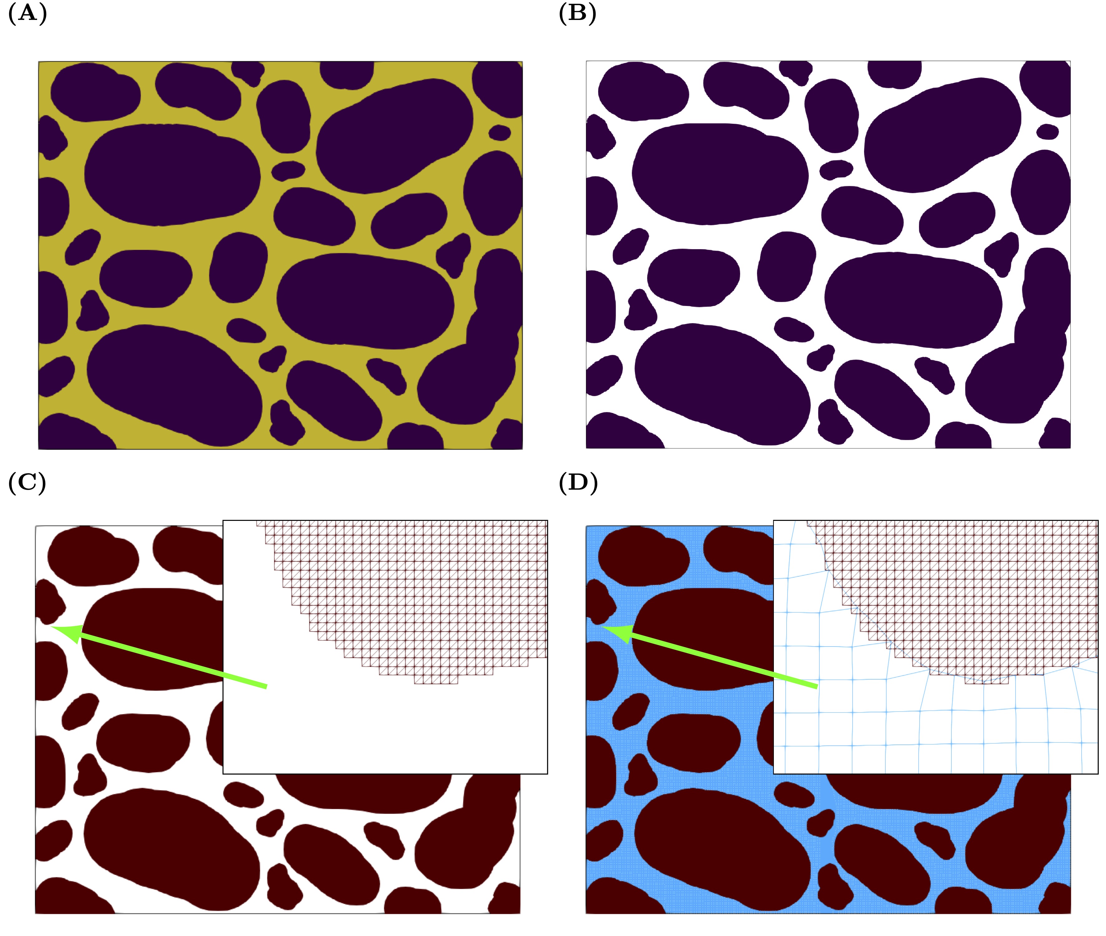
Fig. 7 Workflow illustrating the meshing process.
The steps involved are shown in Fig. 7 . Starting from an image, an stl file is created that is then used during the meshing process. Most of the steps will rely on paraview filters and the workflow is this.
Start with an image (A).
Save it as a .vti file that is easily understood by Paraview. We use porespy for this step.
Load the vti file into paraview and use the clip (B) and triangulation (B) filers to created a surface of the pore space (C).
Save this surface as a stl file
Python pre-processing
Let’s work through the steps involved and assume we received a 2-D image of scanned pore space ( Fig. 7 A). We need to translate it into something that Paraview understands, so that we can do the segmentation and surface generation. We will use porespy for it; make sure it is available in your pyhton environment.
The complete openFOAM case can be downloaded from here .
Copy the case into your shared working directory (probably $HOME/HydrothermalFoam_runs). You need to do this within the docker container (your right-hand shell in Visual Studio Code if you followed the recommended setup).
Check out the directory structure shown in Listing 6.
.
├── 0
│   ├── U
│   └── p
├── a.foam
├── clean.sh
├── constant
│   ├── transportProperties
│   ├── triSurface
│   │   └── porous_model.stl
│   └── turbulenceProperties
├── geometry
│   └── porousModel.png
├── run.sh
└── system
    ├── blockMeshDict
    ├── changeDictionaryDict
    ├── controlDict
    ├── extrudeMeshDict
    ├── fvSchemes
    ├── fvSolution
    ├── meshQualityDict
    └── snappyHexMeshDict
Tip
Most OpenFoam cases include scripts like run.sh and clean.sh. The run.sh script is a good starting point for “understanding” a case. It lists all commands that have to be executed (e.g. meshing, setting of properties, etc.) to run a case. The clean.sh script cleans up the case and deletes e.g. the mesh and all output directories. Have a look into these files and see if you understand them!
Next we import the .png file from the geometry folder and convert it to a .vti file, which is the Visualization Toolkit’s format for storing image data. Note that vti files can also store series of images, which is important when doing this in 3-D.
import numpy as np
from PIL import Image
import porespy as ps
import os

impath = './geometry'         # image path
imname = 'porousModel.png'   # file name

# 1. use PIL to load the image
# convert("L") converts RGB into greyscale, L = R * 299/1000 + G * 587/1000 + B * 114/1000
image = Image.open(os.path.join(impath, imname)).convert("L")

# 2. convert image into numpy array with "normal" integer values
arr = np.asarray(image, dtype=int)

# 3. save as vti (VTK's image format)
# 3.1 make 3D by repeating in new axis=2 dimension (openfoam and porespy want 3D)
arr_stacked = np.stack((arr,arr), axis=2)

# 3.2 save as vti using porespy
ps.io.to_vtk(arr_stacked, 'geometry/porous_model')
You can put this little script into a jupyter notebook or save it as .py (e.g. png2vti.py), then activate the right kernel (e.g. conda activate py312_dome_workshop), and do this:
python png2vti.py
After running it, you should have a file porous_model.vti in the geometry folder.
Tip
If you are interested in the vti file format, this is what we have just written to porous_model.vti. There is a non-zero chance that porespy will write out a binary file and not ascii. If that is the case, you can open it in paraview.
<VTKFile type="ImageData" version="1.0" byte_order="LittleEndian" header_type="UInt64">
    <ImageData WholeExtent="0 1196 0 1494 0 2" Origin="0 0 0" Spacing="1 1 1" Direction="1 0 0 0 1 0 0 0 1">
        <Piece Extent="0 1196 0 1494 0 2">
        <PointData>
        </PointData>
        <CellData Scalars="im">
        <DataArray type="Int64" Name="im" format="ascii" RangeMin="0" RangeMax="255">
            255 255 255 255 255 255
            255 255 255 255 255 255
            255 255 255 255 255 255
            ...
Notice how this is written as cell data. The total extents are 1197x1495x3, the voxel size is 1, and the cell data is 1196x1494x2 (our two images).
Now comes the segmentation and triangulation part to make an stl file that openFOAM understands. We will use paraview for this and there are different ways of doing this:
use paraview’s graphical user interface
use paraview’s inbuild python shell
install paraview into a conda environment and do everything in python scripts or notebooks (the paraview python bindings are called
paraview.simplebut are sometimes a pain to install).
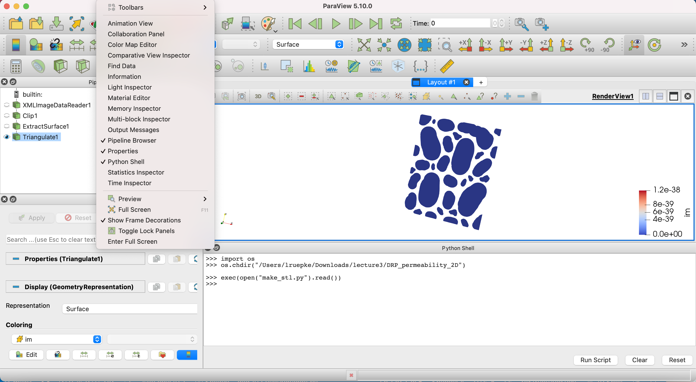
Fig. 8 Using the paraview python shell.
Here is some python code that uses the paraview python bindings. You can save it into your case directory. Or, you use the paraview GUI to create the stl file.
# workflow as python code using the paraview.simple module
# from paraview.simple import * #not needed in paraview's python shell
import os

def write_stl(vti_file, stl_file):
    # 1. load vti file
    data            = OpenDataFile(vti_file)
    # 2. clip at some intermediate value (we have 0 and 255 as pores and grains)
    clip1           = Clip(data, ClipType = 'Scalar', Scalars = ['CELLS', 'im'], Value = 127.5, Invert = 1)
    # 3. make a surface of the remaining grains
    extractSurface1 = ExtractSurface(clip1)
    # 4. and triangulate it for stl export
    triangulate1    = Triangulate(extractSurface1)

    # 5. finally save it as an stl file
    SaveData(stl_file, proxy = triangulate1)

# main part
vti_file = './geometry/porous_model.vti'      # input .vti file
stl_file = './constant/triSurface/porous_model.stl'  # output .stl file
# call function
write_stl(vti_file, stl_file)
An easy way to exectute the python scrip is to save the above code into a file (e.g. write_stl.py) and call it from the python shell in paraview Fig. 8. Within the shell, you first make sure that you are in your case directory; then you make the correct folder to hold the .stl file that we will create (./constant/triSurface).
import os
os.chdir("your_case_directory")
os.mkdir('constant/triSurface')
exec(open("your_file_name.py").read())
This will create a .stl file, which we will use in the meshing process.
If you did not use the python script but did everything step-by-step using the paraview GUI, you might have to do some cleanup, so that the files are in the correct location. Move the vti file into ./geometry and the stl file into ./constant/triSurface, where openFOAM expects it. This assumes that you are in the case directory.
mv ./porous_model.vti ./geometry/
mv ./porous_model.stl ./constant/triSurface/
OpenFOAM case
Making the mesh
Great, back to openfoam for the final mesh making! Making the mesh with SHM is a two-step process. First we make a standard blockMesh background mesh. This is, as usual, controlled by system/blockMeshDict:
  1/*--------------------------------*- C++ -*----------------------------------*\
  2=========                 |
  3\\      /  F ield         | OpenFOAM: The Open Source CFD Toolbox
  4 \\    /   O peration     | Website:  https://openfoam.org
  5  \\  /    A nd           | Version:  7
  6   \\/     M anipulation  |
  7\*---------------------------------------------------------------------------*/
  8FoamFile
  9{
 10    version     2.0;
 11    format      ascii;
 12    class       dictionary;
 13    object      blockMeshDict;
 14}
 15
 16// * * * * * * * * * * * * * * * * * * * * * * * * * * * * * * * * * * * * * //
 17
 18convertToMeters 1;
 19
 20lx0 0;
 21ly0 0;
 22lz0 0;
 23
 24lx1 1196;
 25ly1 1494;
 26lz1 1;
 27
 28vertices
 29(
 30    ($lx0 $ly0 $lz0)   //0
 31    ($lx1 $ly0 $lz0)   //1
 32    ($lx1 $ly1 $lz0)   //2
 33    ($lx0 $ly1 $lz0)   //3
 34    ($lx0 $ly0 $lz1)   //4
 35    ($lx1 $ly0 $lz1)   //5
 36    ($lx1 $ly1 $lz1)   //6
 37    ($lx0 $ly1 $lz1)   //7
 38);
 39
 40blocks
 41(
 42    hex (0 1 2 3 4 5 6 7) (315 390 1) simpleGrading (1 1 1)
 43);
 44
 45edges
 46(
 47);
 48
 49boundary
 50(
 51    top
 52    {
 53        type symmetryPlane;
 54        faces
 55        (
 56            (7 6 3 2)
 57        );
 58    }
 59
 60    inlet
 61    {
 62        type wall;
 63        faces
 64        (
 65            (0 4 7 3)
 66        );
 67    }
 68
 69    bottom
 70    {
 71        type symmetryPlane;
 72        faces
 73        (
 74            (1 5 4 0)
 75        );
 76    }
 77
 78    outlet
 79    {
 80        type patch;
 81        faces
 82        (
 83            (1 2 6 5)
 84        );
 85    }
 86
 87    front
 88    {
 89        type patch;
 90        faces
 91        (
 92            (0 3 2 1)
 93        );
 94    }
 95    back
 96    {
 97        type patch;
 98        faces
 99        (
100            (4 5 6 7)
101        );
102    }
103);
Notice how we set the vertical and horizontal extents to 1196 and 1494, which is the pixel resolution of the image. We will scale it later to physical dimensions. Note how this is actually a 3D mesh, with one cell in the third dimension.
Now have a look at system/snappyHexMeshDict. We will not go into details here, just explore the general structure yourself if you are interested using the resources linked above.
Time to make the mesh! Run each of the steps below individually and check out the results in paraview.
blockMesh
snappyHexMesh -overwrite
Create a temporary file a.foam to load the case into paraview. Also load the stl file to see how well the mesh fits the geometry.
Now we need to make the mesh 2D again for our simulation. This is done by taking the front surface of the 3D mesh and extruding it. Afterwards, we need to set the front and back surface to empty, so that the mesh is truly 2D. This is a bit of a hack, but snappyHexMesh does not do 2D meshes directly.
extrudeMesh
changeDictionaryDict
Both commands read the respective dictionary files from system. The first command extrudes the front surface of the mesh by 1 cell in the z-direction. The second command changes the front and back patches to empty.
Finally, we need to scale the mesh to physical dimensions. We will assume that each pixel in the image is 1 micrometer (\(10^{-6} m\)). This is done using the transformPoints utility.
transformPoints "scale=(1e-6 1e-6 1e-6)"
Boundary conditions
Next we need to set boundary conditions. Our “rock” sample is 1196 and 1494 \(\mu m\) and we will apply a constant pressure drop of 1 Pa. We will further use openFOAM’s simpleFoam solver, which resolves incompressible steady-state flow. One important thing to remember is that openFOAM uses the kinematic pressure in incompressible simulations, which is the pressure divided by density. If we assume that water with a density of \(1000kg/m^3\) is flowing through our example, we will need to set a constant pressure value of \(P_{left}=0.001 m^2/s^2\). The pressure on the right-hand side will be set to zero.
Open the file p inside the 0 directory from your local left-hand shell.
code 0/p
 1/*--------------------------------*- C++ -*----------------------------------*\
 2=========                 |
 3\\      /  F ield         | OpenFOAM: The Open Source CFD Toolbox
 4 \\    /   O peration     | Website:  https://openfoam.org
 5  \\  /    A nd           | Version:  7
 6   \\/     M anipulation  |
 7\*---------------------------------------------------------------------------*/
 8FoamFile
 9{
10    version     2.0;
11    format      ascii;
12    class       volScalarField;
13    location    "0";
14    object      p;
15}
16// * * * * * * * * * * * * * * * * * * * * * * * * * * * * * * * * * * * * * //
17
18dimensions      [0 2 -2 0 0 0 0];
19
20internalField   uniform 0;
21
22boundaryField
23{
24    top
25    {
26        type            symmetryPlane;
27    }
28    inlet
29    {
30        type            fixedValue;
31        value           uniform 0.001;
32    }
33    bottom
34    {
35        type            symmetryPlane;
36    }
37    outlet
38    {
39        type            fixedValue;
40        value           uniform 0;
41    }
42    solids
43    {
44        type            zeroGradient;
45    }
46    frontAndBack
47    front
48    {
49        type            empty;
50    }
51    back
52    {
53        type            empty;
54    }
55}
The boundary conditions are again set for the patches that were defined in the blockMeshDict. Notice how the sides have constant values. The top and bottom are symmetry planes and the internal boundaries with the solid grains get a zeroGradient condition. As we are performing a 2-D simulations, the front and back faces are set to empty.
Remember that units are set by the dimensions keyword. The entries refer to the standard SI units [Kg m s K mol A cd]. By having a 2 in the second and third column, we get the correct units for the kinematic pressure.
We also need to set boundary conditions for the velocity.
code 0/U
 1/*--------------------------------*- C++ -*----------------------------------*\
 2=========                 |
 3\\      /  F ield         | OpenFOAM: The Open Source CFD Toolbox
 4 \\    /   O peration     | Website:  https://openfoam.org
 5  \\  /    A nd           | Version:  7
 6   \\/     M anipulation  |
 7\*---------------------------------------------------------------------------*/
 8FoamFile
 9{
10    version     2.0;
11    format      ascii;
12    class       volVectorField;
13    location    "0";
14    object      U;
15}
16// * * * * * * * * * * * * * * * * * * * * * * * * * * * * * * * * * * * * * //
17
18dimensions      [0 1 -1 0 0 0 0];
19
20internalField   uniform (0 0 0);
21
22boundaryField
23{
24    top
25    {
26        type            symmetryPlane;
27    }
28    inlet
29    {
30        type            zeroGradient;
31    }
32    bottom
33    {
34        type            symmetryPlane;
35    }
36    outlet
37    {
38        type            zeroGradient;
39    }
40    solids
41    {
42        type            noSlip;
43    }
44    front
45    {
46        type            empty;
47    }
48    back
49    {
50        type            empty;
51    }
52}
The top and bottom are again symmetry planes and the zeroGradient condition ensure that fluids can freely flow in and out. The contacts with the solid grains get noSlip, which makes the velocity go to zero; front and back are again set to empty.
Transport properties
Final step is to set the remaining free parameter (viscosity) in equation ().
code constant/transportProperties
 1/*--------------------------------*- C++ -*----------------------------------*\
 2=========                 |
 3\\      /  F ield         | OpenFOAM: The Open Source CFD Toolbox
 4 \\    /   O peration     | Website:  https://openfoam.org
 5  \\  /    A nd           | Version:  7
 6   \\/     M anipulation  |
 7\*---------------------------------------------------------------------------*/
 8FoamFile
 9{
10    version     2.0;
11    format      ascii;
12    class       dictionary;
13    object      transportProperties;
14}
15// * * * * * * * * * * * * * * * * * * * * * * * * * * * * * * * * * * * * * //
16
17transportModel  Newtonian;
18
19nu              [0 2 -1 0 0 0 0] 1e-06;
20
21// ************************************************************************* //
Again, in incompressible simulations (where we can divide the momentum balance equation by density) the kinematic viscosity is used, which has units of \(m^2/s\). The value of \(1e{-6} m^2/s\) with an assumed density of \(1000kg/m^3\) is \(1 mPa\) - a typical value for water at room temperature.
Case control
Finally, we need to set some control parameters in system/controlDict. Open it and explore the values.
code system/controlDict
 1/*--------------------------------*- C++ -*----------------------------------*\
 2=========                 |
 3\\      /  F ield         | OpenFOAM: The Open Source CFD Toolbox
 4 \\    /   O peration     | Website:  https://openfoam.org
 5  \\  /    A nd           | Version:  7
 6   \\/     M anipulation  |
 7\*---------------------------------------------------------------------------*/
 8FoamFile
 9{
10    version     2.0;
11    format      ascii;
12    class       dictionary;
13    object      controlDict;
14}
15// * * * * * * * * * * * * * * * * * * * * * * * * * * * * * * * * * * * * * //
16
17application     simpleFoam;
18
19startFrom       startTime;
20
21startTime       0;
22
23stopAt          endTime;
24
25endTime         1500;
26
27deltaT          1;
28
29writeControl    timeStep;
30
31writeInterval   1500;
32
33purgeWrite      0;
34
35writeFormat     ascii;
36
37writePrecision  9;
38
39writeCompression off;
40
41timeFormat      general;
42
43timePrecision   6;
44
45runTimeModifiable true;
The solver is a stead-state solver, so that the settings are quite simple with respect to transient simulations.
Running the case
Now we are finally ready to run the case! Just type this into your docker shell:
./run.sh
or, if you did the steps above by hand:
simpleFoam
Notice how one new directory is appearing, which contains the steady-state solution. Check that the solution has converged by looking at the log.simpleFoam file.
tail -15 tail -15 log.simpleFoam

Time = 536s

smoothSolver:  Solving for Ux, Initial residual = 8.33332294e-10, Final residual = 8.33332294e-10, No Iterations 0
smoothSolver:  Solving for Uy, Initial residual = 9.84562833e-10, Final residual = 9.84562833e-10, No Iterations 0
GAMG:  Solving for p, Initial residual = 9.67603673e-09, Final residual = 9.67603673e-09, No Iterations 0
time step continuity errors : sum local = 7.10016507e-07, global = -1.23478036e-07, cumulative = 4.09450688
ExecutionTime = 24.158663 s  ClockTime = 25 s


SIMPLE solution converged in 536 iterations

End
And explore the solution in Paraview!
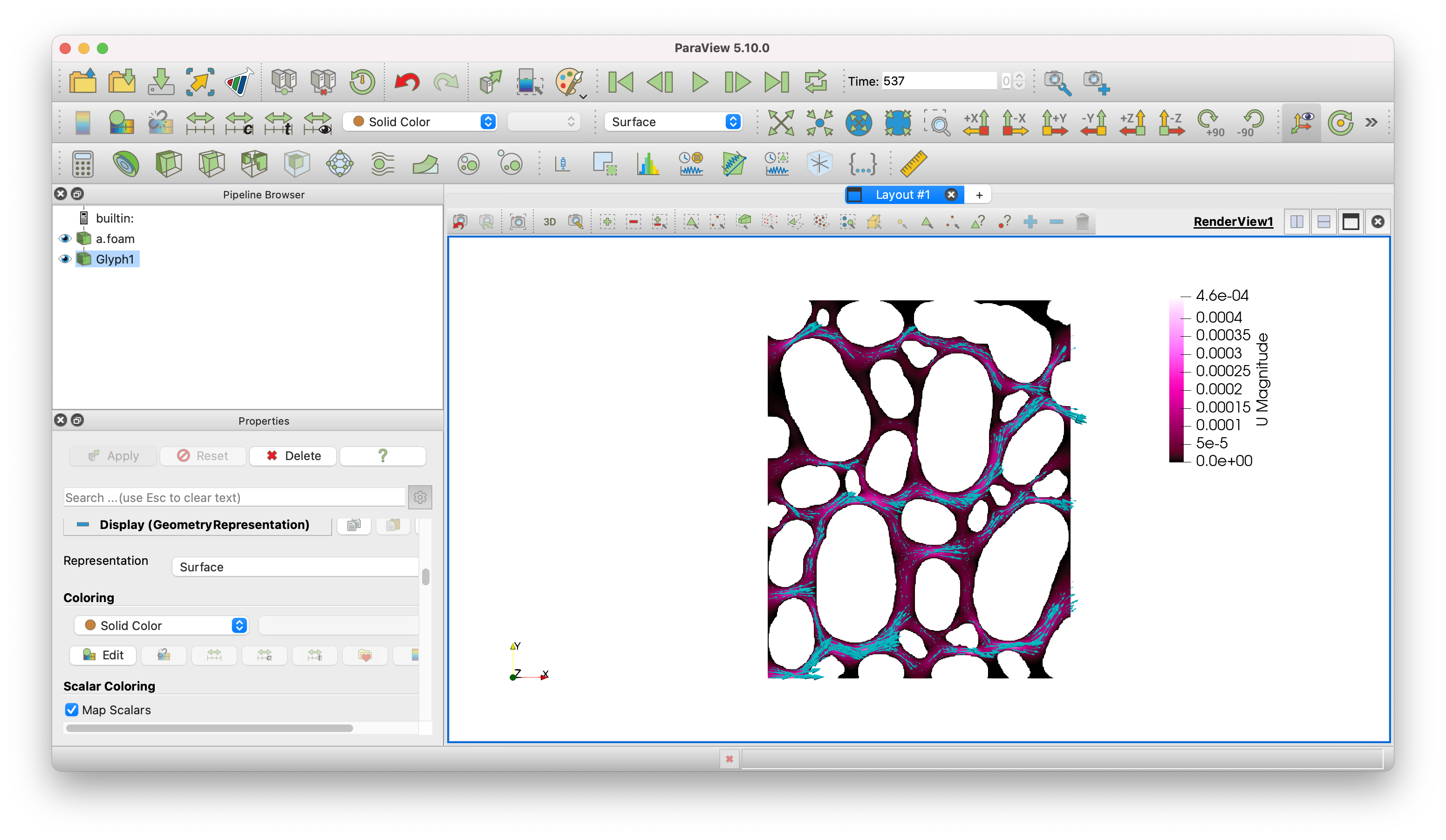
Fig. 9 Predicted velocity field.
Post-processing / Effective permeability
Time to get back to our initial objective. What is the predicted permeability of our sample? We need to postprocess our solution and solve equation (), which requires are few intermediate steps. First, we need to compute the cell volumes, so that we can integrate the velocity over the total volume. Here comes openFOAM’s postProcess functionality handy. Just do this:
postProcess -func writeCellVolumes
This will create a new variable \(V\) in in the output directories, which is the volume of each cell. Next we can save the full solution as a vtk file, so that we can postprocess it with python.
foamToVTK -useTimeName -latestTime -poly
Check that a new VTK directory was created. Now we are ready for some more fancy post-processing using python.
Here is an example script for computing permeability. You can turn it into a jupyter notebook or save it as a .py file into your case directory and run it from there.
import vtk
import numpy as np
from vtk.util import numpy_support as VN
import matplotlib.pyplot as plt

# load VTK data
vtkFile = 'VTK/DRP_permeability_2D_536.vtk'
reader = vtk.vtkUnstructuredGridReader()
reader.SetFileName(vtkFile)
reader.ReadAllScalarsOn()
reader.ReadAllVectorsOn()
reader.Update()
data = reader.GetOutput()


# extract velocity arrays
Vcells = VN.vtk_to_numpy(data.GetCellData().GetArray('V'))
U = VN.vtk_to_numpy(data.GetCellData().GetArray('U'))
Umag = np.sqrt(U[:,0]**2+U[:,1]**2+U[:,2]**2)
Ux = U[:,0]
Uy = U[:,1]
Uz = U[:,2]

# calculate volume fluxes
qx = []
qy = []
for c in range(len(Vcells)):
    q1 = Vcells[c] * Ux[c]
    q2 = Vcells[c] * Uy[c]
    qx.append(q1)
    qy.append(q2)

# simulation parameters
DP = 1                       # pressure drop [Pa]
nu = 1e-06                   # kinematic viscosity [m²/s²]
rho = 1000                   # density [kg/m³]
mu = nu * rho                # dynamic viscosity [kg/(m*s)]
dx = 0.001196                # model length x [m]
dy = 0.001494                # model width y [m]
dz = 1e-6                    # model thickness z [m]
A = dy * dz
V = dx * A

# calculate Darcy velocity
U_Darcy_x = np.sum(qx)/V

kxx = mu * dx * U_Darcy_x/DP

print('Bulk permeability: %5.3e m2' % kxx)
We made it! \(2.71e^{-11} m^2\) is our predicted effective permeability of our sample.