Navier-Stokes flow with OpenFoam

In this lecture we will solve the famous Navier-Stokes equation for flow. There are many different forms of the Navier-Stokes equations, depending on the assumptions made. Her we solve the form that is treated in the icoFoam solver in OpenFOAM. It treats incompressible, laminar, and transient fluid flow and solves the following equations:

\[\frac{\partial \mathbf{U}}{\partial t} + (\mathbf{U} \cdot \nabla)\mathbf{U} = -\nabla p + \nu \nabla^2 \mathbf{U}\]

\[\nabla \cdot \mathbf{U} = 0\]

where:

\(\mathbf{U}\) is the velocity vector field,
\(p\) is the kinematic pressure (i.e., pressure divided by density),
\(\nu\) is the kinematic viscosity,
\(t\) is time.

The first equation is the momentum conservation equation:

\(\partial \mathbf{U} / \partial t\) represents unsteady acceleration (how velocity changes over time),
\((\mathbf{U} \cdot \nabla)\mathbf{U}\) is the advection (fluid moving itself),
\(-\nabla p\) is the pressure gradient force,
\(\nu \nabla^2 \mathbf{U}\) is the viscous diffusion of momentum.

The second equation enforces incompressibility, meaning the volume of fluid elements does not change over time.

In icoFoam, these equations are solved using the finite volume method and the PISO algorithm (Pressure Implicit with Splitting of Operators) to ensure pressure–velocity coupling and divergence-free velocity fields at each time step. We will get into the details of the numerical methods later in the course. For now, we will just use the solver and its capabilities.

2D cavity flow

Our first example of simulating Navier-Stokes flow is flow within a 2D cavity. Flow is driven by a kinematic boundary condition at one side, while all other sides are walls with zero velocity. The model setup is shown in Fig. 3 .

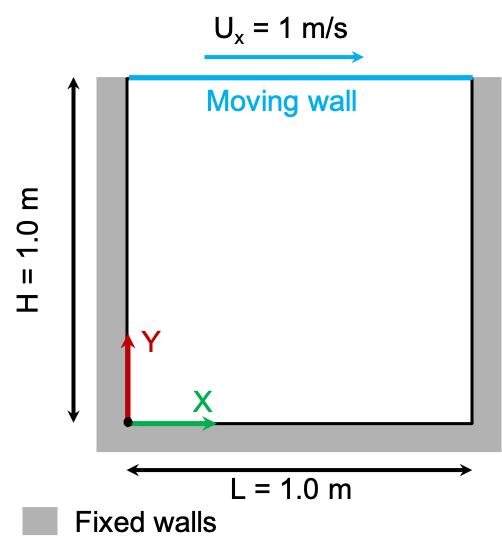
../../_images/2d_cavity_setup.png — Fig. 3 Two-dimensional cavity model geometry and boundary conditions. Note a mistake in the figure: the domain size is actually 0.1 m by 0.1 m in the tutorial.

Preparing the case

Two-dimensional cavity flow is included in the official tutorials of OpenFoam. We get started by copying the tutorial case into our work directory. You need to do this from your docker shell.

cd $HOME/HydrothermalFoam_runs
cp -r $FOAM_TUTORIALS/incompressible/icoFoam/cavity/cavity ./cavity2D

Check the directory structure:

.
├── 0
│   ├── U
│   └── p
├── a.foam
├── clean.sh
├── constant
│   └── transportProperties
└── system
    ├── blockMeshDict
    ├── controlDict
    ├── fvSchemes
    └── fvSolution

The 0 directory now contains the boundary and initial conditions for pressure and velocity (our primary variables), the constant directory has the transport properties (here viscosity), and the system directory contains information on the mesh, time steps, numerical schemes etc.

The two files run.sh and clean.sh are actually not included and we need to create them. These files are usually part of every OpenFoam case; run.sh includes all commands that need to executed to run the case and clean.sh cleans the case (removes mesh and output directories).

Listing 6 The run.sh file.

#!/bin/sh
cd ${0%/*} || exit 1    # Run from this directory

# Source tutorial run functions
. $WM_PROJECT_DIR/bin/tools/RunFunctions

application=`getApplication`

./clean.sh
runApplication blockMesh
runApplication $application

Listing 7 The clean.sh file.

#!/bin/sh
cd ${0%/*} || exit 1 # run from this directory

# Source tutorial run functions
. $WM_PROJECT_DIR/bin/tools/CleanFunctions

# Clean the case
cleanCase

Make the scripts executable.

chmod u+x clean.sh run.sh

Making the mesh

We will use OpenFoam’s blockMesh utility to make a simple 2D mesh. The corresponding blockMeshDict file that has all the meshing information is located in the system folder.

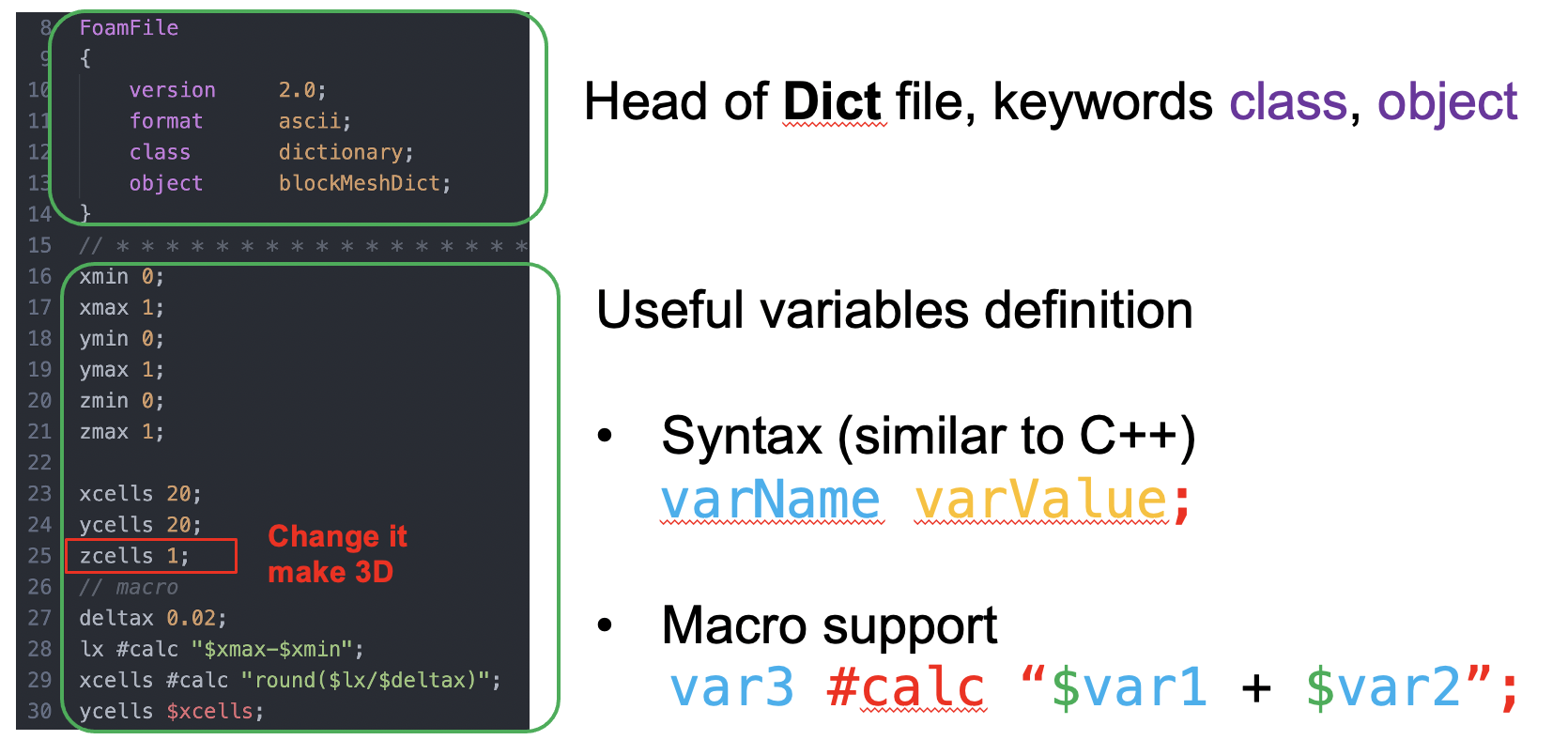
../../_images/cavity2d_bm.png — Fig. 4 Structure of the blockMeshDict

First we need to define the vertices of the mesh, the nodes.

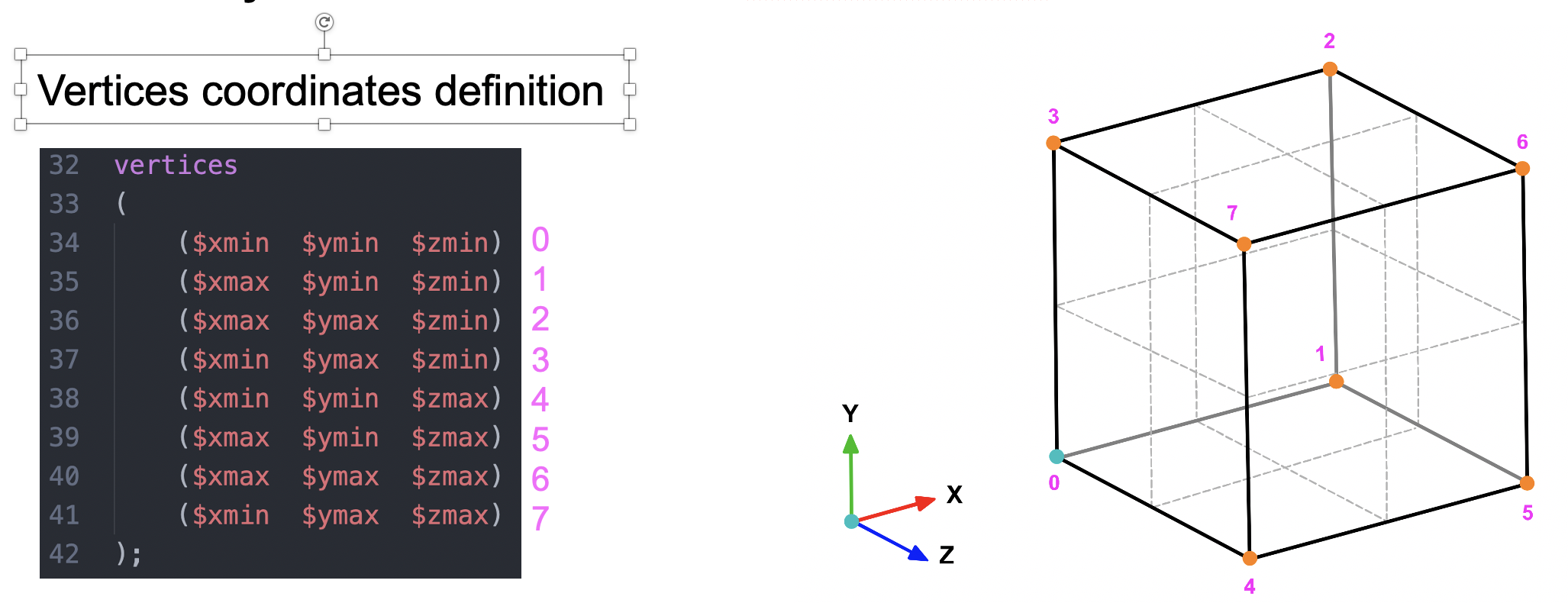
../../_images/cavity2d_vertices.png — Fig. 5 Numbering of the vertices.

The next step is define the connectivity between the vertices in order to describe the modeling domain.

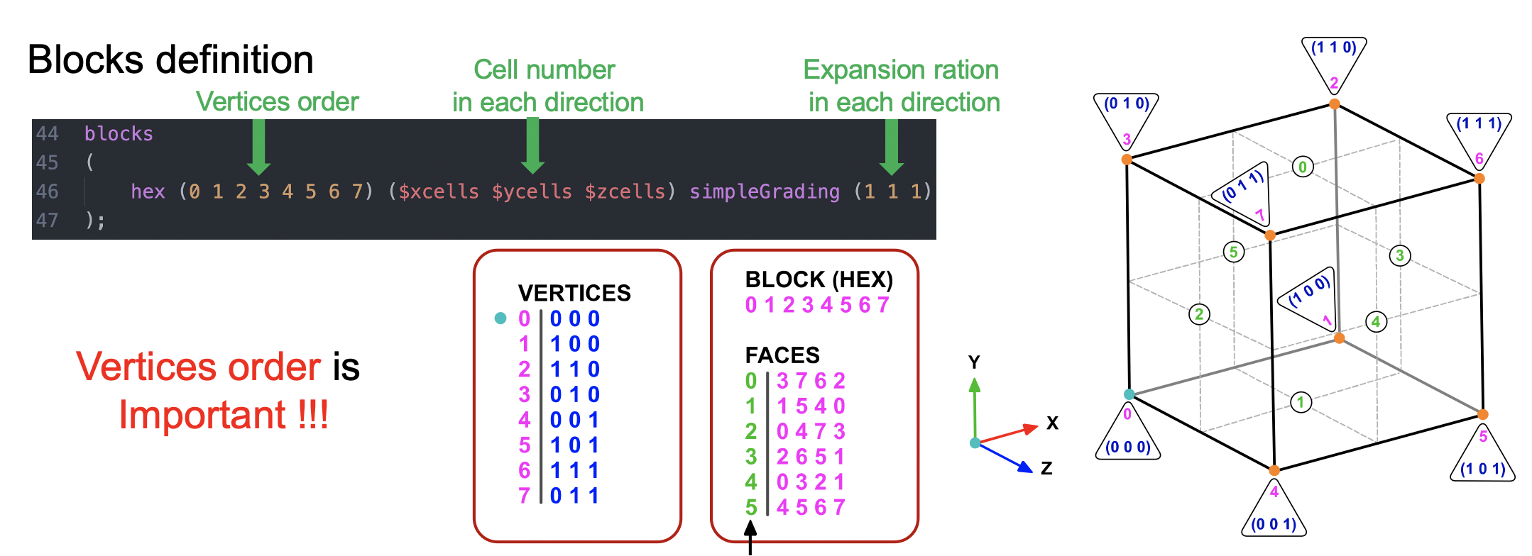
../../_images/cavity2d_vorder.png — Fig. 6 The order by which the vertices are passed to the hex command matters!

Order of vertices

The OpenFoam documentation provides a nice description of the vertices ordering.

the axis origin is the first entry in the block definition, vertex 0 in our example
the x direction is described by moving from vertex 0 to vertex 1
the y direction is described by moving from vertex 1 to vertex 2
vertices 0, 1, 2, 3 define the plane z = 0
vertex 4 is found by moving from vertex 0 in the z direction
vertices 5,6 and 7 are similarly found by moving in the z direction from vertices 1,2 and 3 respectively.

Next boundary patches are defined and labeled in the blockMeshDict. Also here care must be take to provide the vertices in a consistent order (right-hand coordinate system). Two easy ways to remember this is to:

apply the right-hand rule, which means if the thumb of your right hand points to the outside of a face, the numbering has to follow your fingers.

or, looking onto a face and starting from any vertex, the numbering has to be counter-clockwise.

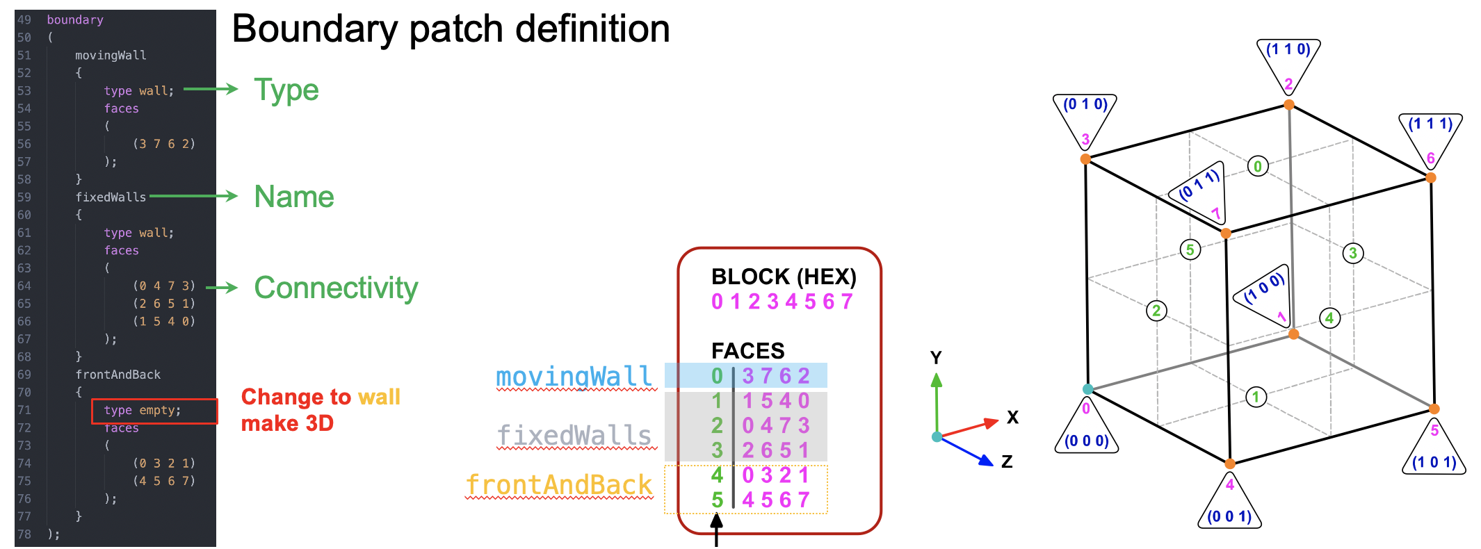
../../_images/cavity2d_bounds.png — Fig. 7 Assigning boundary labels and types.

Now we are ready to run the blockMesh utility and create the mesh

blockMesh

You can visualize the mesh using paraview

touch a.foam
paraview a.foam

Boundary conditions

We now have velocity and pressure as primary variables and need to set initial and boundary conditions for them. First we look at the velocity boundary conditions:

code 0/u

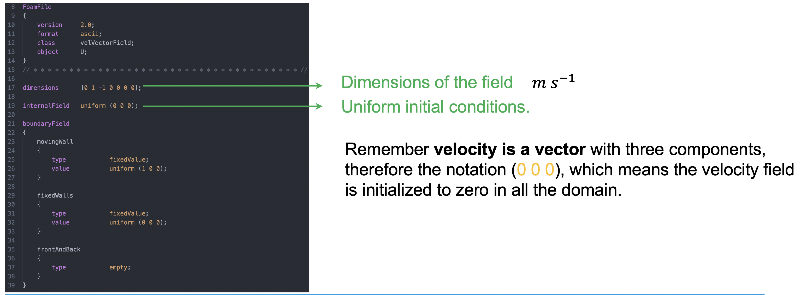
../../_images/cavity2d_u.png — Fig. 8 Velocity boundary conditions. The front and back sides are set to empty because we are doing a 2D calculation.

Next we look into the pressure boundary conditions.

code 0/p

Listing 8 Pressure boundary conditions. Front and back are of type “emtpy” for 2-D runs.

/*--------------------------------*- C++ -*----------------------------------*\
=========                 |
\\      /  F ield         | OpenFOAM: The Open Source CFD Toolbox
 \\    /   O peration     | Website:  https://openfoam.org
  \\  /    A nd           | Version:  7
   \\/     M anipulation  |
\*---------------------------------------------------------------------------*/
FoamFile
{
    version     2.0;
    format      ascii;
    class       volScalarField;
    object      p;
}
// * * * * * * * * * * * * * * * * * * * * * * * * * * * * * * * * * * * * * //

dimensions      [0 2 -2 0 0 0 0];

internalField   uniform 0;

boundaryField
{
    movingWall
    {
        type            zeroGradient;
    }

    fixedWalls
    {
        type            zeroGradient;
    }

    frontAndBack
    {
        type            empty;
    }
}

// ************************************************************************* //

Tip

One has to be careful about the dimensions of pressure in OpenFoam. In incompressible runs, like we are doing here, the pressure is usually the relative pressure \(\frac{p}{\rho}\) and has units \(\frac{m^2}{s^2}\)

Run controls

The time stepping, run time, and output frequency are again set in system/controlDict. Open it and check that you understand the entries.

Listing 9 controlDict of the cavity flow tutorial.

/*--------------------------------*- C++ -*----------------------------------*\
=========                 |
\\      /  F ield         | OpenFOAM: The Open Source CFD Toolbox
 \\    /   O peration     | Website:  https://openfoam.org
  \\  /    A nd           | Version:  9
   \\/     M anipulation  |
\*---------------------------------------------------------------------------*/
FoamFile
{
    format      ascii;
    class       dictionary;
    location    "system";
    object      controlDict;
}
// * * * * * * * * * * * * * * * * * * * * * * * * * * * * * * * * * * * * * //

application     icoFoam;

startFrom       startTime;

startTime       0;

stopAt          endTime;

endTime         0.5;

deltaT          0.005;

writeControl    timeStep;

writeInterval   20;

purgeWrite      0;

writeFormat     ascii;

writePrecision  6;

writeCompression off;

timeFormat      general;

timePrecision   6;

runTimeModifiable true;


// ************************************************************************* //

Here is a short explanation of the most important entries:

application: Solver used (here, icoFoam for incompressible laminar flow).
startFrom: Start method (startTime = use value from startTime).
startTime: Initial simulation time.
stopAt: Stop method (endTime = use value from endTime).
endTime: Final simulation time.
deltaT: Time step size.
writeControl: When to write output (timeStep = every N time steps).
writeInterval: Write output every N time steps.
purgeWrite: Max number of saved time steps (0 = keep all).
writeFormat: Output file format (ascii or binary).
writePrecision: Number of digits in numerical output.
writeCompression: Compress output files (off or on).
timeFormat: Time label format (e.g., general, fixed).
timePrecision: Precision of time labels.
runTimeModifiable: Allow runtime dictionary edits (true = yes).

These are the most important entries. There are many more options available, which can be found in the OpenFoam User Guide

In case you wondered how OpenFoam is solving the equations. We will cover the details later in the course, but you can have a preview by opening the system/fvSchemes file. In this dictionary, the various discretization schemes can be set. Fig. 9 gives some further explanations.

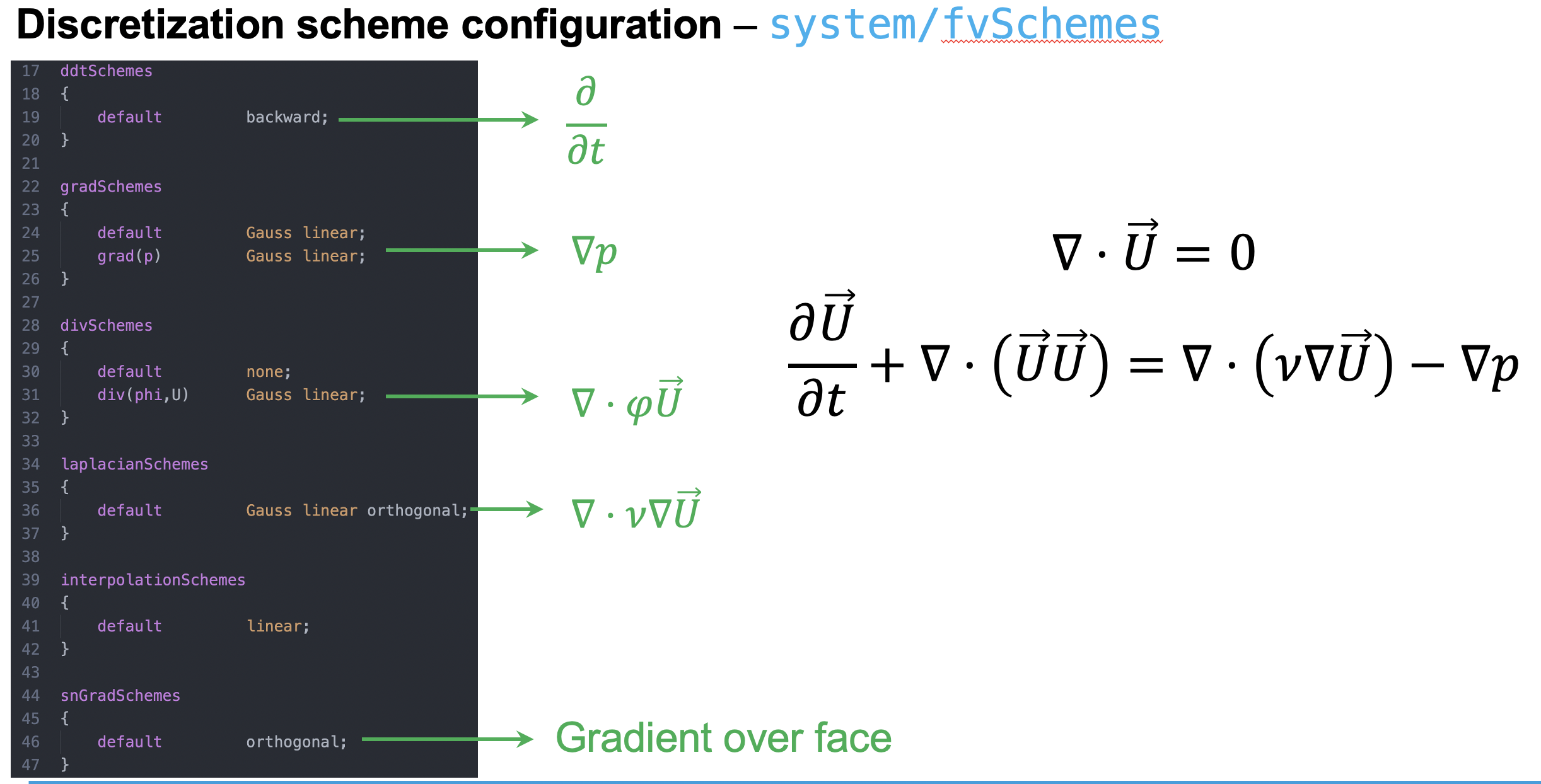
../../_images/cavity2_num.png — Fig. 9 The exact discretization schemes can be set in `system/fvSchemes`.

Time to run the case! Just start the solver

icoFoam

Visualization

Open paraview and look at the results. They are actually quite boring because the flow is steady and laminar; and because we have not first thought about the expected results. Let’s do that better in the the next excercise.