Script for calculating steady state 1D advection-diffusion using FDM methods

import numpy as np
import numpy.matlib
from scipy.linalg import solve
from scipy.sparse import spdiags
import matplotlib.pyplot as plt
from matplotlib import animation
from IPython.display import HTML
import matplotlib as mpl
mpl.rcParams['figure.dpi']= 300

# model parameters
c       = 20
k       = 2
nx      = 11
x0      = 0
x1      = 1

Tleft   = 0
Tright  = 1

X,dx    = np.linspace(x0,x1, nx, retstep=True)

#peclet number for stability analysis
peclet  = c*dx/(2*k)

#analytical solution with boundary conditions T(0) = 0 and T(1) = 1;
C2      = 1/(1-np.exp(c/k))
C1      = -C2;
Tana    = C1*np.exp(c/k*X) + C2

# hide
# FTCS solution
# build the coefficient matrix
data  = (np.ones((nx,1))*np.array([-(c/(2*dx) + k/dx**2), (2*k/dx**2), -(-c/(2*dx)+k/dx**2) ])).T
diags = np.array([-1, 0, 1])
A     = spdiags(data, diags, nx, nx).toarray()

# and add boundary conditions
A[0,0]       = 1
A[0,1]       = 0
A[nx-1,nx-1] = 1
A[nx-1,nx-2] = 0

Rhs          = np.zeros(nx)
Rhs[0]       = Tleft
Rhs[-1]      = Tright

Tftcs=solve(A,Rhs)

## FTCS solution
## build the coefficient matrix
#data  = (np.ones((nx,1))*np.array([???, ???, ??? ])).T
#diags = np.array([-1, 0, 1])
#A     = spdiags(data, diags, nx, nx).toarray()

## and add boundary conditions
#A[0,0]       = 1
#A[0,1]       = 0
#A[nx-1,nx-1] = 1
#A[nx-1,nx-2] = 0
#Rhs          = np.zeros(nx)
#Rhs[0]       = Tleft
#Rhs[-1]       = Tright
#Tftcs=solve(A,Rhs)

# hide
# upwind solution
# build the coefficient matrix
data  = (np.ones((nx,1))*np.array([-(c/dx + k/dx**2), (c/dx+2*k/dx**2),  -k/dx**2 ])).T
diags = np.array([-1, 0, 1])
A     = spdiags(data, diags, nx, nx).toarray()

# and add boundary conditions
A[0,0]       = 1
A[0,1]       = 0
A[nx-1,nx-1] = 1
A[nx-1,nx-2] = 0
Tuw=solve(A,Rhs)

## upwind solution
## build the coefficient matrix
#data  = (np.ones((nx,1))*np.array([???, ???,  -???])).T
#diags = np.array([-1, 0, 1])
#A     = spdiags(data, diags, nx, nx).toarray()

## and add boundary conditions
#A[0,0]       = 1
#A[0,1]       = 0
#A[nx-1,nx-1] = 1
#A[nx-1,nx-2] = 0
#Tuw=solve(A,Rhs)

# Create the figure and axis
fig, ax = plt.subplots(figsize=(10, 5))

# Set axis limits
ax.set_xlim(x0, x1)
ax.set_ylim(min(Tleft, Tright, Tana.min(), Tftcs.min(), Tuw.min()), max(Tleft, Tright, Tana.max(), Tftcs.max(), Tuw.max()))

# Set axis labels
ax.set_xlabel('Distance', fontsize=14)
ax.set_ylabel('Temperature', fontsize=14)

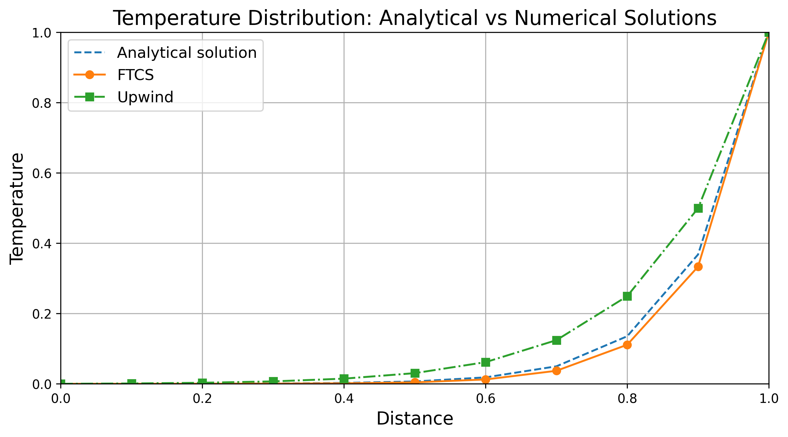
# Plot the analytical and numerical solutions
ax.plot(X, Tana, label='Analytical solution', linestyle='--')
ax.plot(X, Tftcs, label='FTCS', linestyle='-', marker='o')
ax.plot(X, Tuw, label='Upwind', linestyle='-.', marker='s')

# Add a legend
ax.legend(fontsize=12)

# Add a title
ax.set_title('Temperature Distribution: Analytical vs Numerical Solutions', fontsize=16)

# Add a grid for better readability
ax.grid(True)

# Show the plot
plt.show()