Exercises
Let’s explore the solution in a bit more detail.
Vertical versus horizontal permeability
Make a copy of your case and repeat the analysis in the vertical direction. You will need to
adapt the face types in blockMeshDict
modify the boundary conditions in
0/pand0/Umodify the post-processing script to compute vertical velocity
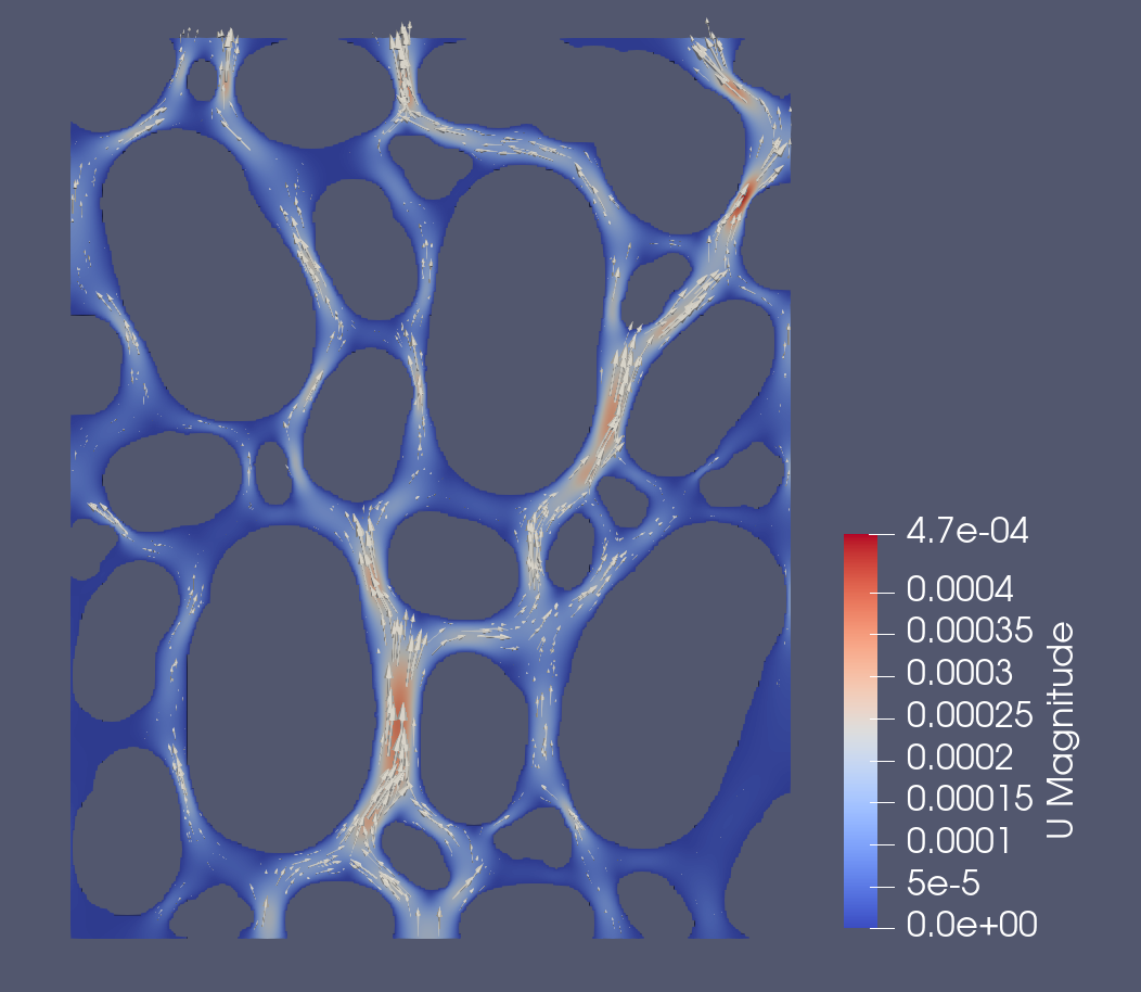
You should get something like this:

Fig. 15 Pore-level flow in the vertical direction.
Changes to the geometry
Check if/how the solution changes if you distort the mesh. For example, squeeze it a bit in the vertical direction by modifying the transformPoints -scale "(1e-6 1e-6 1e-6)" statement. Also check if the absolute dimensions matter!
Numerical models should (usually) not surprise us. So before running the different case, ask yourself what you expect.
will permeability increase or decrease if you squeeze the sample, for example by half in one direction?
Do the absolute dimension matter?
Adding scalar transport
In the next session, we will progress towards submarine hydrothermal systems and will explore Darcy flow in detail. In preparation for that, let’s explore how scalar transport (like advecting temperature) would look like in our synthetic pore model.
OpenFOAM’s scalarTransportFoam application solves the 3-D advection-diffusion equation for a given velocity field:
with T being the transported scalar, DT the diffusivity with units of \(m^2/s\) , and ST is a source term. Note that it is tempting to think of T as temperature but here it is simply a transported scalar (like a solute in groundwater flow). The energy conservation equation written in terms of temperature looks slightly different, as we will learn in the next chapter.
The key source code of scalarTransportFoam looks like this:
...
fvScalarMatrix TEqn
(
    fvm::ddt(T)
    + fvm::div(phi, T)
    - fvm::laplacian(DT, T)
    ==
    fvModels.source(T)
);

TEqn.relax();
fvConstraints.constrain(TEqn);
TEqn.solve();
fvConstraints.constrain(T);
...
Since we have already computed the velocity field (and made the mesh etc.), we can now use our results as the starting point for a scalarTransportFoam case. The foam tuturials are always a good starting point for a new case. scalarTransportFoam is handled in $FOAM_TUTORIALS/basic/scalarTransportFoam/pitzDaily/ . Let’s copy it over to our working directory, add our velocity field and mesh, and modify the control dictionoaries.
In the docker do this:
cd $HOME/HydrothermalFoam_runs
cp -r $FOAM_TUTORIALS/basic/scalarTransportFoam/pitzDaily/ ./DRP_transport
cp -r ./DRP_permeability_2D/constant/polyMesh ./DRP_transport/
cp ./DRP_permeability_2D/0/U ./DRP_transport/0/
This assumes that you used the case and directory names; if not, modify the names accordingly.
Now go back to our local shell and Visual Studio and modify the scripts:
0/Tto make “temperature” 1 at the inlet and zeroGradient at the outlet
constant/transportPropertiesset the diffusivity to something small, like \(1e-{12}\), so that the problem is advection-dominatedchange
system/controlDictso that the endTime is 20, deltaT is 0.1, and writeInterval is 3e-1. These are somewhat arbitrary changes making sure we get a reasonable solution for our synthetic setup.
That’s it, run it and explore the solution!
Would the temperature evolution in our rock sample look like this? What would the grains do the speed of the thermal front?